Optimization

During the design process, commissioning, and operation of products and systems, optimization is an important step in solving engineering problems. Solving optimization problems using the REPEAT VISION platform allows you to:

1. Design units with maximum Efficiency;

2. Perform optimal design of process systems to improve production efficiency;

3. Effectively adapt calculation models to the diagnostic results of operating products to reduce decision-making risks through the ability to conduct virtual tests.

 In the process of system modeling, the tasks listed above are reduced to determining the parameters of the blocks so that the calculation model operates in an optimal state. For example:

• Find the value of the parameter at which the output signal of the system becomes zero (root finding problem);

• Select several parameters simultaneously to minimize or maximize an objective function that calculates, for example, the Efficiency of a unit (local or global optimization).

 The Optimization tool, located in the bottom panel (see Fig. 1 below), simplifies this process. You don’t need to manually iterate through the values—the optimizer itself interacts with the calculation model and selects parameters following a specified algorithm.

Fig. 1 Optimization tool

1.  Operating principle

1. You formulate an optimization problem and define the objective function for optimization.

2. You create a model, configure it, and debug it.

3. You configure the task by selecting the optimization type, budget (number of model calls), algorithm, and search boundaries.

4. You run the calculation—the optimizer calls the calculation model as many times as allowed by the budget, analyzing the results and refining the parameters.

5. Get the result - in the results table you can see the current and proposed values, and then you can apply them to the model.

2.  Interface

 Optimization settings areas (see Fig. 2 below):

• Main settings:

  • Optimization task type;

  • Optimization budget;

  • Handling of non-physical values (NaN).

• Optimization algorithm:

  • Root finding method;

  • Absolute tolerance of the varied param…

Note

The algorithm settings depend on the selected task type

• Parameter settings:

  • Optimized parameters - selection of block parameters to be optimized.

  • Variable properties - selection of changeable block properties.

• The Optimize button starts the process.

Hint

When in doubt, it’s best to start with local optimization. Global requires more computing resources.

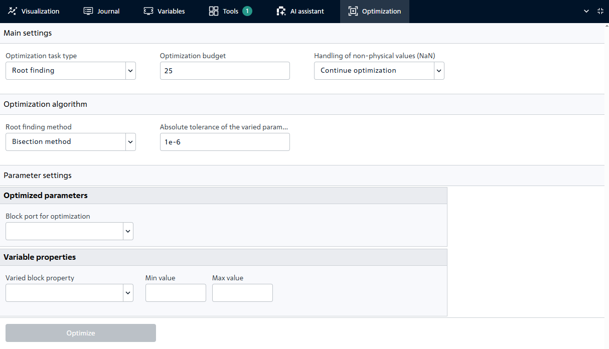
Fig. 2 Optimization settings zones

2.1.  Optimization budget

 The budget is the number of times the optimizer will evaluate the computational model. Each time the algorithm calculates the objective function, the budget is reduced by 1. When the budget is exhausted, optimization stops.

Budget value selection table

Example	Recommended budget
Simple model (calculated in a fraction of a second), root search	20-50
Complex model (seconds to calculate), local optimization	50-200
Global optimization (requires many iterations)	200-1000
Debugging and testing	10-20

Hint

If the budget is 0, optimization will not make any requests. Use only to test logic.

2.2.  Setting up the algorithm

 This group of fields depends on the selected optimization task type (Main settings section). The fields for each type are described below:

Root finding

• Root finding method:

  • The Bisection method is the most stable method for finding the root, the disadvantage of which is the large computational budget and, as a consequence, (relative to Brent's method) a long time to solve the problem.

  • The Brent's method provides a fast solution to the root finding problem.

• Absolute tolerance of the varied parameter is the real value of the convergence criterion of the optimizer for the absolute value of the deviation of the variable parameter.

Local optimization

Additionally, an Optimization method is selected. It is the method that determines whether the problem being solved is one-dimensional or multidimensional:

Метод оптимизации	Тип задачи	Что делает
Ограниченный метод	Одномерная	Оптимизация функции одной переменной с ограничениями (границами)
Метод Нелдера-Мид	Многомерная	Оптимизация функции множества переменных

 The user explicitly selects the method, and the problem type (univariate/multivariate) is determined automatically.

Global optimization

• Root finding method - Differential evolution.

• Population size is a multiplier used to determine the total population size. The total population size is determined by multiplying the population size by the number of variable parameters.

Размер популяции	Поведение
4-8	Быстро, но риск пропустить глобальный минимум
10-20	Хорошо для большинства задач
>20	Медленно, используйте только для сложных многомерных задач

• Random seed - is specified to generate a set of pseudo-random numbers in order to ensure repeatability of the results of the stochastic optimization algorithm.

• Initial guess of the parameter to speed up the search for the optimal value. Can only be within the boundary of the variable parameter. Can be equal to a value smaller or larger than the boundary of the variable parameter.

2.3.  Optimized parameters

 This is the value that the optimizer is trying to minimize, maximize, or reduce to zero. This is the optimization objective.

2.4.  Variable properties

 This is a property of a block in the diagram whose value the optimizer can change during the search process. These are control levers.

Note

• For Root finding and Local optimization (Limited Method), the user can select only one property.

• For Local optimization (Nelder-Mead method) and Global optimization, you can select multiple properties (up to 20).

2.5.  Launch optimization

 When you click the Optimize button, the form is checked again and if there are no errors, the optimization calculation is started.

 When Optimization is running, a button to stop Optimization appears to the right of the Optimize button - Cancel, which interrupts the Optimization calculation process if it takes too long and the user wants to interrupt it.

 Once optimization is complete, the user will see a message with a link to the results.

2.6.  Optimization results

 The Results section appears only after the first successful calculation. When you run optimization again, the old table is completely replaced by the new one; the results of the previous calculation are not saved.

The results table contains the following columns:

Column	Description
Parameter	The name of the parameter or port that was involved in the optimization
Current value	What was set in the model before running the optimization
Suggested value	What the algorithm found. This is the value that the optimizer believes is best suited to achieving the goal (the root, minimum, or maximum).
Range	The boundaries within which the solution was allowed to be searched. These were set by the user when configuring the variable properties.
Apply	A checkbox appears next to each parameter. It allows you to select which suggested values ​​you want to apply and which to ignore. The user selects the checkboxes next to the parameters they want to change and clicks the “Apply Selected” button.

Hint

• A simpler and faster option is to click Apply All - and all suggested values ​​will be applied immediately, without the need to check boxes.

• You can simply look at the results, close the tab, and leave everything as is. The optimization is already complete, and the model remains unchanged. This is a normal scenario—for example, when you’re just studying an algorithm’s behavior or comparing different approaches.

3.  Examples of use

 Examples of using this tool can be found in the following sections:

• Tutorials;

• How-to guides.

Tutorials

Library	Tutorial name
Solving optimization problems	Introduction to Optimization; Finding the root

How-to guides

Section	Guide name
Solving optimization tasks	Determining the required water flow rate in a pipeline system