

Finding the root#
One of the common categories of optimization problems solved in engineering practice is the inverse problem, which consists of determining the value of \(x\) for which the equality (1) is satisfied.
The canonical form of the equality (1), known from the school mathematics course for solving the problem of finding the zeros of a function, has the form \(f(x) = 0\).
Hint
It is worth recalling the direct problem, which consists of calculating the value \(y = f(x)\) for a known parameter \(x\).
This tutorial will examine a typical formulation of the problem of finding the root of the objective function, during which you will become familiar with:
With examples of inverse problems in engineering calculations;
With a simple formulation of the root search problem to acquire skills in solving inverse problems using the Optimization of the REPEAT VISION platform.
1. Statement of the problem of finding the root of the objective function#
The problem of finding the root is formulated as follows:
The following notation is used in the root finding problem (2):
\(f\) is the objective function for which we need to find the root \(x\) when \(f(x) = 0\);
\(g\) is the function for which \(x\) must be found when \(g(x) = \text{const}\);
\(\text{const}\) is the known value of the function \(g\);
\(x\) - objective function parameter (or design point),
\(\chi\) is the set of admissible values of the function parameter.
The value \(x\) that belongs to \(\chi\) and for which the objective function \(f(x) = 0\) is the root of the equation (2), denoted by \(x^{*}\).
In the root finding problem (2), the parameter \(x\) can be either a scalar represented as a real number (double in Java) or a vector represented as a set of \(n\) real numbers (3).
2. Examples of inverse problems#
The technical specifications (TS) for the design of a new system may include the task of determining previously unknown values of the system parameters for compliance with the required technological characteristics of the system. For example, determine the diameter of the throttle orifice - \(x [mm]\) in (1) - to ensure the required water flow rate - \(\text{const} [kg/s]\) in (1) - in the pipeline system. This requirement TS determines the formulation of the inverse problem and the need to find the root \(x\) to solve the problem.
Examples of inverse problems related to root finding are listed in the table below.
Task |
Modeling areas |
|---|---|
Defining the required flow rate of a liquid in a pipeline system |
|
Selecting a pump for a pipeline system |
|
Determining the value of the LED current-limiting resistor |
The inverse problems from the table above often do not have an exact analytical solution.
Previously, inverse problems were solved by conducting a computational experiment on a model of the system. Computational experiment is the process of repeatedly performing a system simulation to solve a direct problem. At the beginning of each iteration of the computational experiment, the input parameters \(x\) model are changed, and at the end of the simulation, the results \(f(x)\) of the calculation are collected. The experiment cycle is terminated when the equality (1) is satisfied with the specified error. This approach has a number of disadvantages for solving the inverse problem:
Engineer manually changes the input parameters $x$, runs {term}model
for calculation, analyzes the results and checks the equality {eq}baserootfind`;It takes a lot of working time to find a solution to \(x^{*}\) problem;
The {bdg-danger-line} engineer
empiricallyregulates the step of changing the parameters \(x\), often not providing an exact solution to the \(x^{*}\) problem;
To eliminate the above mentioned shortcomings, it is necessary to use modern methods for solving inverse problems, which are available in the Optimization of the REPEAT VISION platform.
In the next section, we will consider a typical formulation of the problem of finding the root of the objective function.
3. Example of an inverse problem#
In this section, we consider a function of the form \(g(x) = \sqrt[2]{x}\) for \(x \in [0; 400]\). We need to find \(x\) of the function \(g\) such that \(g(x) = 15\). This simple formulation of the inverse problem will allow us to focus on acquiring skills in working with the Optimization of the REPEAT VISION platform.
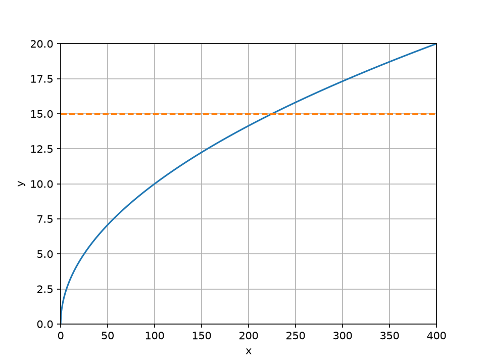
The function whose root needs to be found#
The following notations are used in the graph above.
Lines |
Description |
|---|---|
Blue line |
Function \(g(x) = \sqrt[2]{x}\), \(x \in [0; 400]\) |
Orange line |
Auxiliary function \(y = 15\) to indicate where \(x\) needs to be found at the intersection with \(g(x)\) |
3.1. Analytical solution#
For the problem \(\sqrt[2]{x} = 15\), the exact analytical solution is known, \(x^{*}= 225\).
3.2. Creating a model in REPEAT VISION#
To create a model for finding the root of a objective function on the REPEAT VISION platform, it is necessary to transform the inverse problem to the form (2). Thus, the original task of finding \(x\) will take the form \(f(x) = \sqrt[2]{x} - 15\). The Optimization will search for the root of the objective function, checking for the equality \(f(x) = 0\).
To prepare the model, you need to add 4 blocks of the Automation library to a new project named, for example, Square Root.
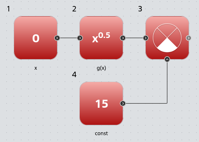
Root finding model for the objective function in REPEAT VISION#
First, a block №1 Constant is added to the project with the Constant value property equal to 0. This block will be used as the parameter \(x\) (see equation (2)) of the objective function \(f(x)\).
Then block №2 Raising to the constant power is added, with the Power property set to 0.5. This block will be used to extract the square root, \(\sqrt[2]{x}\).
Next, block №3 Signal difference (Controller error) is added to the project. This block is used to calculate the objective function \(\sqrt[2]{x} - 15\) together with block #4. In accordance with the problem statement of root finding (2), this block will be used by the optimizer to check the equality \(f(x) = 0\).
To complete the model preparation, it is necessary to add block №4 Constant with the Constant value property equal to 15 in accordance with the problem statement.
Important
In each problem of finding the root \(x\) of the objective function \(f(x) = g(x) - \text{const} = 0\), a pair of blocks is needed to perform this operation:
A constant to fix the value \(\text{const}\) that the function \(g(x)\) should take;
A comparator for performing the subtraction operation \(g(x) - \text{const}\) in order to verify that \(f(x) = 0\) when searching for the root of the objective function by the optimizer.
For this stationary problem statement, it will be sufficient to use the following project settings:
Simulation time \([s]\) |
Integration step \([ms]\) |
Sampling step \([ms]\) |
|---|---|---|
0.1 |
50 |
50 |
In the next section, we configure the optimizer to obtain a solution to the root problem.
3.3. Configuring the optimizer#
To configure the Optimization, you need to click on the ‘Optimization’ icon on the bottom panel.
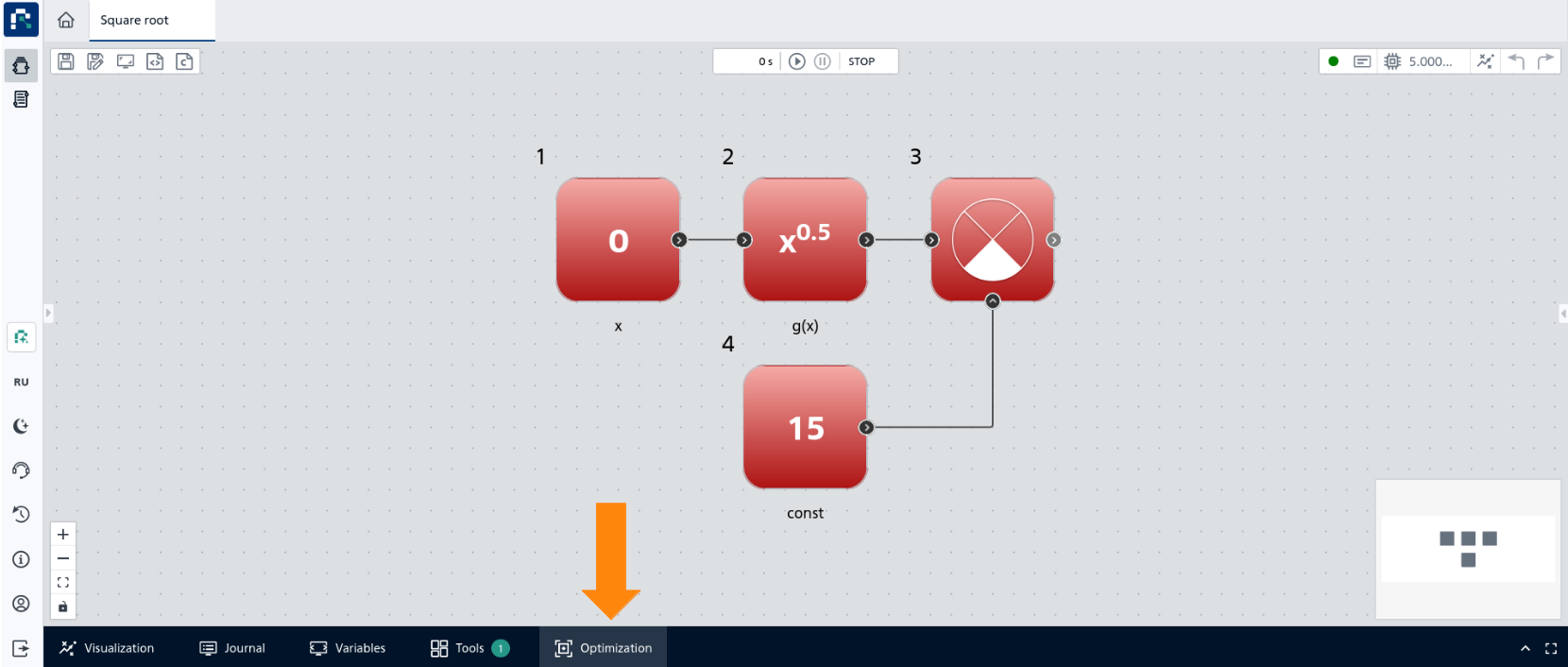
The location of the Optimization icon on the bottom panel of the REPEAT VISION interface#
In the tab that opens, you need to apply the settings to solve the root search problem.
Main settings#
In the Main settings section, you need to apply the following settings.
Optimization task type |
Optimization budget |
Handling of non-physical values (NaN) |
|---|---|---|
Finding the root |
25 |
Raise exception |
Optimization budget is the number of available optimizer calls to the computational model for calculating the objective function. Each time the algorithm passes the next value of the parameter \(x\) to the objective function and receives a new value of the objective function \(f(x)\) in response, the budget decreases by 1. When the budget is exhausted, the root search is forced to stop.
Hint
For simple, smooth, continuous objective functions similar to quadratic functions, a small budget (\(10 \leq budget \leq 100\)) is sufficient to solve the root finding problem.
In the Handling of non-physical values (NaN) setting, you should select Raise exception since in a simple model there will be no problems with calculating the objective function that could lead to errors during modeling. Therefore, there is no need for additional processing of the calculation results with checking for the physicality of the results of calculating the objective function.
Optimization algorithm#
In the Optimization algorithm section, you need to apply the following settings.
Optimization method |
Absolute tolerance of the varied parameter |
|---|---|
Brent’s method |
1e-15 |
In the Optimization method setting, you must select Brent's method to search for the root using the Brent method, which guarantees the convergence of the solution to the problem for the objective function, computable within the specified boundaries.
The setting Absolute tolerance of the varied parameter must be assigned a value of 1e-15 to fix the convergence criterion for the solution of the optimization problem for the parameter \(x\).
Note
It should be noted that the small value of 1e-15, close to the precision of a double in Java, is suitable for Brent's method and smooth, continuous objective functions.
Parameter settings#
In the Objective function calculation block setting, located in the Optimized parameters section, you must select the Output port of block №3 Raising to the constant power, which performs the final operation of calculating the objective function \(f(x)\).
In the Varied block property setting, located in the Variable properties section, you must select the Constant value property of block №1 Constant. The value of the block constant will be used by the optimizer as a variable parameter \(x\) to find the root of the objective function \(f(x)\) (see equation (2)).
You also need to specify the boundaries within which to search for the root. In the current example, the boundaries of the objective function are taken to be \(x \in [0; 400]\). So, in the Min value field you need to enter 0, and in the Max value field you need to enter 400.
4. Start optimization#
After completing the optimizer setup, you need to run the optimization. To start optimization, you need to click on the Optimize button
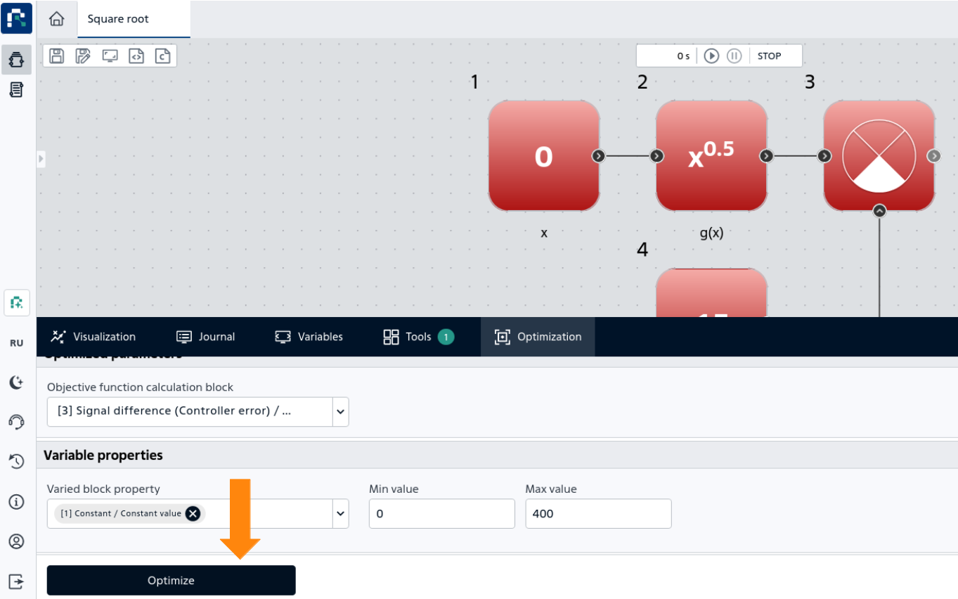
Click the Optimize button to start optimization.#
After clicking the button, notifications about the start of optimization and the successful completion of optimization will appear (#pic_popup_opt).
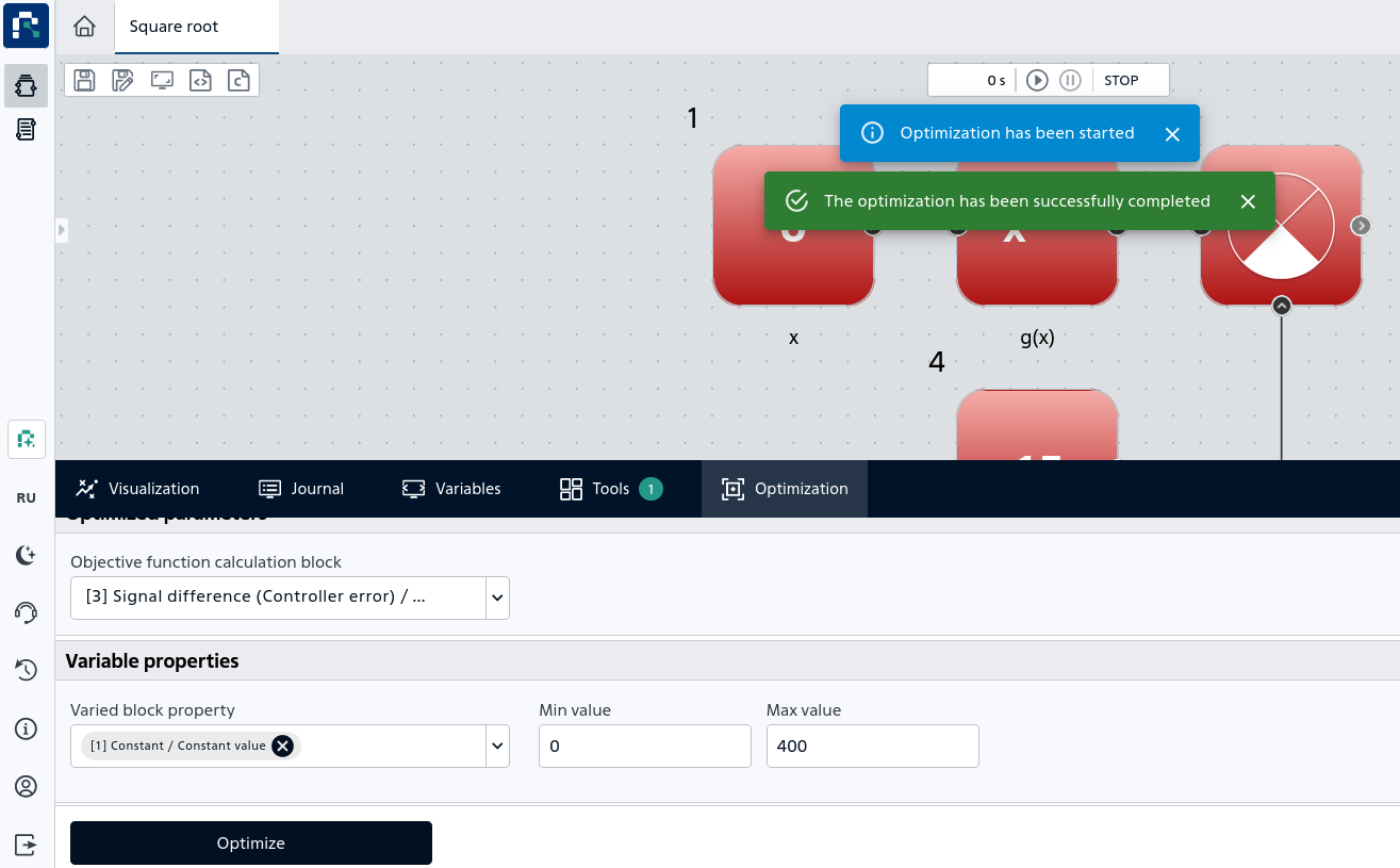
Notifications of the stages of the root search process#
After successfully completing the root search, it is necessary to analyze the obtained solution.
4.1. Analysis of optimization results#
The optimization results are available in the corresponding section for performing analysis after successful completion of the root search.
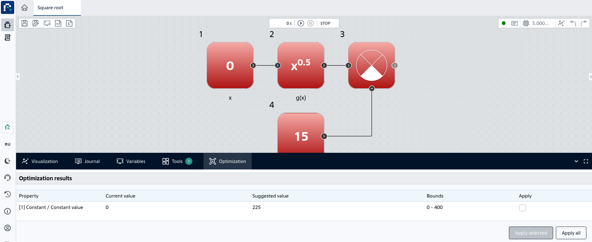
Root search results#
The optimizer determined the root of the objective function \(f(x)\) for the parameter \(x\) equal to 225, which corresponds to the exact analytical solution.
Next, you need to click on the Apply all button to transfer the root of the target function \(x^{*} = 225\) to the Constant value property of block №1 Constant. After clicking the button, a notification will appear indicating that the optimal properties have been successfully applied.
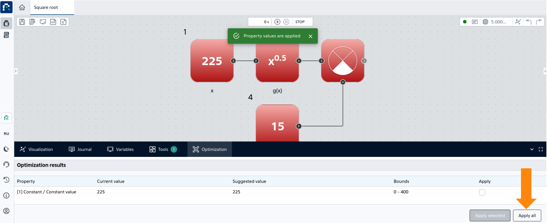
Application to the model of optimal properties#
At the end of the analysis, it is necessary to run the calculation of the model with the root value \(x^{*} = 225\) and get the calculation result on the Output port of block №3 Signal difference (Controller error), which performs the final operation of calculating the objective function \(f(x)\).
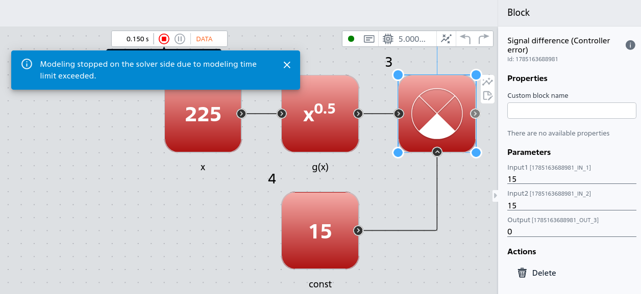
The value of the objective function at x = 225.#
The calculation result shows:
The value of the objective function \(f(x^{*}) = 0\) at the
Outputport of block №3,The value of the function \(g(x^{*}) = 15\) on the port
Input 1of block №3
with the value of the parameter \(x^{*} = 225\), which corresponds to the exact analytical solution.
5. Conclusions#
As a result of completing the introductory tutorial on solving the root finding problem, you learned:
On the concept of an inverse problem and its place in optimization;
On the method of transforming the inverse problem into the problem of finding the root;
On the objective function for solving root finding problems;
Using a simple example, we mastered the Optimization of the REPEAT VISION platform for solving root finding problems.