

Construction of the flow-pressure characteristics of the network#
1. Introduction#
Design and analysis of thermal hydraulic systems are an integral part of engineering practice in heat power engineering, water supply and many other industries. The key tool for assessing the performance and efficiency of such systems is the flow-pressure characteristic (FPC) of the network. This dependence of the total pressure losses in the network on the flow rate of the working medium allows us to determine the required performance of the pumping equipment and ensure its coordinated operation with the hydraulic circuit.
2. Statement of the problem#
This tutorial examines the practical problem of constructing such a characteristic for a specific thermal hydraulic network. The system consists of a pump that pumps water between two reservoirs with given parameters, and includes linear sections of polypropylene pipelines, local resistances in the form of bends and a filter with known nominal losses, Fig. 1:
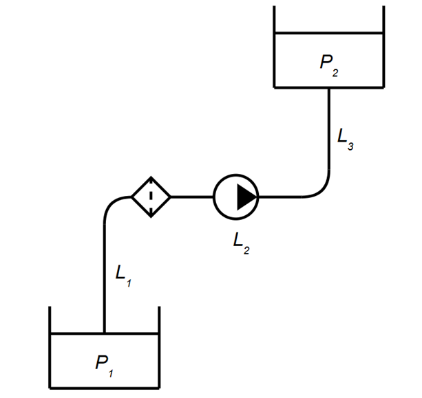
Fig. 1 The hydraulic network under study#
3. Target and tasks#
3.1. Target#
3.2. Tasks#
Create a calculation model of a given hydraulic network in the REPEAT VISION environment, including tanks, pipeline sections and local resistances (branches, filter).
Correctly configure the properties of all network elements (geometric dimensions, absolute roughness, nominal pressure losses, etc.).
Perform a series of hydraulic calculations of the network for different values of mass flow rate and obtain the corresponding values of total pressure losses (required head).
Construct a graph of the network’s FPC based on the calculated points.
To study the application of the FPC network using the example of determining the operating point of the selected pumping equipment.
4. Preparing the calculation model#
To construct the network characteristics, it is necessary to reproduce the hydraulic network without a pumping unit using modeling blocks:
Place the following blocks from the
Thermohydraulicslibrary in the modeling area (see Fig. 2 below):
Tanks and accumulators:Reservoir (TL)- 2 pcs.-
Elbow (TL)- 2 pcs.;Pipe (TL)- 3 pcs.
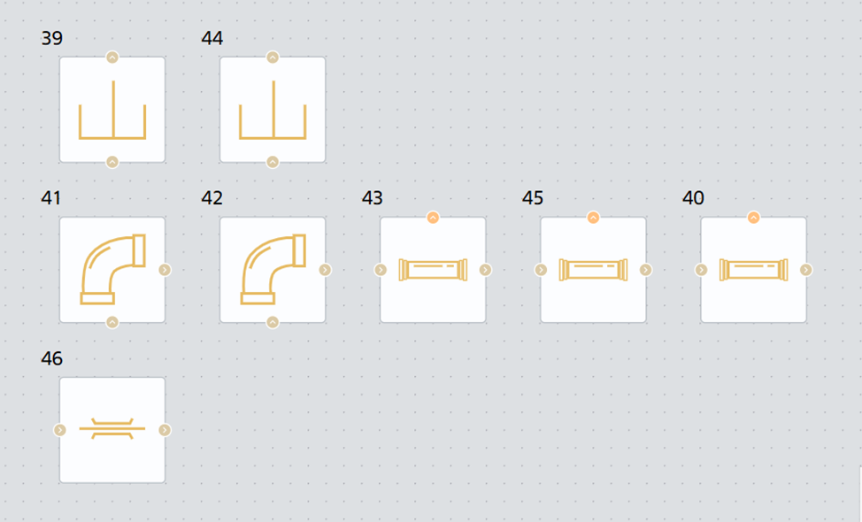
Fig. 2 Necessary blocks#
Add appropriate labels to the blocks as shown in Fig. 3:
Note
The Custom block name is added in the block properties in the field of the same name Custom block name
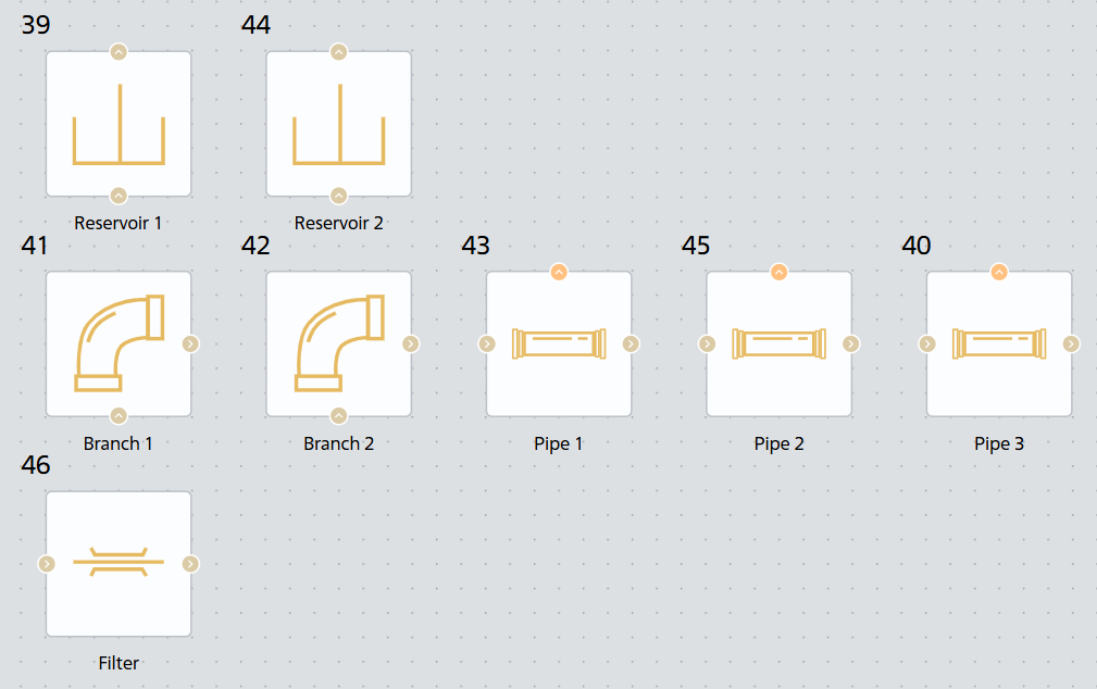
Fig. 3 Blocks with labels#
Connect the blocks as shown in Fig. 4. Rotate them if necessary using the rotation handle.
Hint
The rotation marker  appears when you click on the LMB block
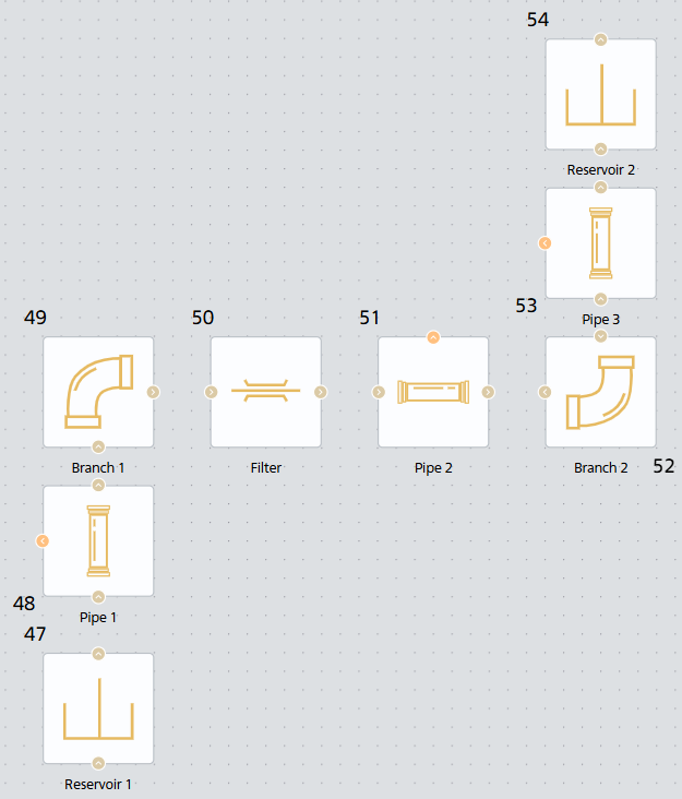
Fig. 4 Hydraulic network model#
To construct a FPC hydraulic network, it is necessary to carry out a series of calculations and see what pressure drop occurs. To perform a series of calculations, we add a Ideal flow rate source (TL) block between tank 1 and pipeline 1 and a differential Pressure and temperature sensor (TL) between the ideal flow source and tank 2 (see Fig. 5 below). The properties of the Pressure and temperature sensor (TL) block are presented in Fig. 6.
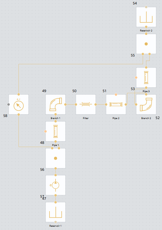
Fig. 5 Hydraulic network with flow source and pressure sensor#
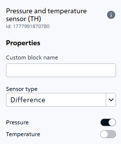
Fig. 6 Properties of the Pressure and temperature sensor (TL) block#
4.1. Filling block properties#
Tables 1–5 show the block properties. If a block property is not listed in a table, its default value is retained.
Table 1 – Properties for Pipe (TL) blocks
Property/Custom block name |
Pipeline 1 |
Pipeline 2 |
Pipeline 3 |
|---|---|---|---|
Pipe length, m |
4 |
2 |
2 |
Pipe diameter, m |
|||
Internal surface absolute roughness, m |
1e-5 |
1e-5 |
Important
In REPEAT VISION, decimal numbers are specified using a dot.
Table 2 – Properties for Elbow (TL) blocks
Property/Custom block name |
Branch 1 |
Branch 2 |
|---|---|---|
Hydraulic diameter, m |
Table 3 – Properties of the Flow resistance (TL) block
Property/Custom block name |
Filter |
|---|---|
Nominal pressure drop, MPa |
|
Nominal mass flow rate, kg/s |
|
Ports cross-sectional area, m |
Table 4 – Properties of the Ideal flow rate source (TL) block
Property/Block |
Ideal flow rate source (TL) |
|---|---|
Mass flow rate, kg/s |
massFlowRate |
Power added |
None |
Ports cross-sectional area, m² |
Table 5 – Properties for Reservoir (TL) blocks
Property/Block |
Reservoir 1 |
Reservoir 2 |
|---|---|---|
Gauge pressure, Pa |
reservoir1GaugePressure |
reservoir2GaugePressure |
Ports cross-sectional area, m |
5. Parametric studies#
The detailed process of preparing models and conducting parametric studies is described in the section Work automation with REPEAT VISION model, check out this tutorial.
During the parametric studies we will vary the flow rate in the network, so it is necessary to create a global variable for this value. Let’s create it in the Variables tab of the bottom panel (see Fig. 7 below). We will also create variables for excess pressure in the tanks to take into account their differences when constructing the network characteristics.
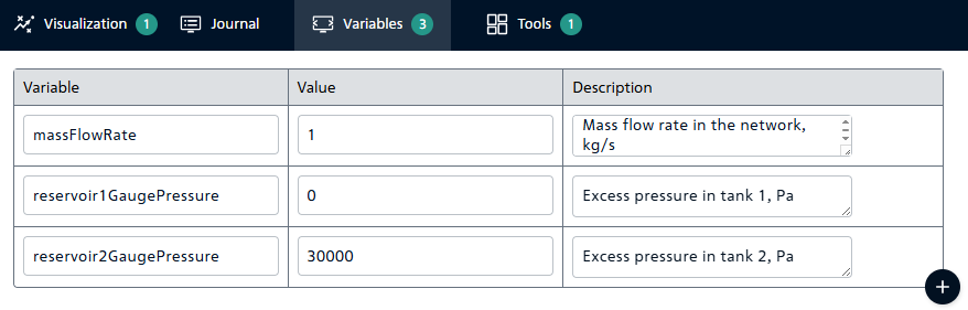
Fig. 7 Global variables of the model#
In addition, we need to get the values of the pressure drop in the system at different flow rates from JupyterLite, so we need to add the Outport block. Let’s add it and connect it to the pressure port of the Pressure and temperature sensor (TL) block (pressureDrop is selected as the user name), Fig. 8:
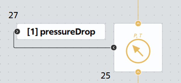
Fig. 8 Output port for receiving data on pressure drop on hydraulic network elements#
Below is the code for the JupyterLite notebook with comments.
Implementation of a series of calculations
# Импорт piplite (пакет Python, который позволяет устанавливать пакеты в блокнотах Jupyter Notebooks) и установка пакета repeat для работы.
import piplite
await piplite.install("repeat")

# Импорт необходимых библиотек
import numpy as np
import pandas as pd
import repeat as rp

# Добавление API ключа в настройки пользователя класса User
user = rp.User(token = 'Your private API key')
# Настройка класса Application для соединения с REPEAT VISION
app = rp.Application(user)
# Сохранение id проекта в отдельную переменную
project = 140501
# Настройка временного интервала для получения значений результатов моделирования
t_interval = rp.TimeInterval(start = 10, end = 1000)
# Создание экземпляра класса Model для получения результатов расчета из модели REPEAT VISION
model = app.get_exploration_model(project, t_interval)

# Переменные в исследуемой модели
existing_vars = model.existing_variables
print(existing_vars)

# Создаем диапазон значений для massFlowRate
mass_flow_rates = np.linspace(0., 0.7, num=20, dtype=float)
results = []  # Список для сохранения результатов
# Значения переменных для избыточных давлений в резеруарах
reservoir1GaugePressure = 0.0
reservoir2GaugePressure = 30000.0
# Цикл для выполнения серии расчетов
for mass_flow in mass_flow_rates:
    # Создаем объект Series со значением текущего расхода
    current_variable = pd.Series({'massFlowRate': mass_flow, 'reservoir1GaugePressure': reservoir1GaugePressure,'reservoir2GaugePressure': reservoir2GaugePressure,}, dtype=float)
    # Запуск расчета модели
    with model as md:
        md.run(current_variable)
        #Сохранение результатов одного расчета в pressureDrop
        pressure_drop = md.get_results('pressureDrop')
    # Сохраняем последнее значение и добавляем разницу давлений в резервурах
        if not pressure_drop.empty:
            last_value = pressure_drop.iloc[-1] + reservoir2GaugePressure - reservoir1GaugePressure
        else:
            last_value = np.nan  # Используем NaN для отсутствующих значений
    results.append((mass_flow, last_value)) # Добавление значений в список

# Создаем DataFrame из списка кортежей
results_df = pd.DataFrame(
    results,
    columns=['massFlowRate', 'pressureDrop']
)
print(results_df)
Data visualization
# Импортируем и устанавливаем необходимые библиотеки для визуализации
import matplotlib.pyplot as plt
await piplite.install("seaborn")
import seaborn as sns

def plot_pressure_drop_curve(results_df, figsize=(10, 6)):
    """
    Создает график зависимости потерь давления от массового расхода.

    Parameters:
    -----------
    results_df : pd.DataFrame
        DataFrame с колонками 'massFlowRate' и 'pressureDrop'
    figsize : tuple
        Размер графика в дюймах (ширина, высота)
    """

    # Настройка стиля графика
    plt.style.use('seaborn-v0_8-dark')

    # Создаем фигуру и оси с указанным размером
    fig, ax = plt.subplots(figsize=figsize, dpi=100)

    # Фильтруем данные, исключая NaN значения для чистоты графика
    clean_data = results_df.dropna(subset=['pressureDrop'])
    # Проверяем, есть ли данные для отображения
    if len(clean_data) == 0:
        print("Нет данных для построения графика (все значения NaN)")
        return

    # Создаем основной график - линию с маркерами
    # Используем маркеры 'o' для точек и линию для соединения
    ax.plot(clean_data['massFlowRate'],
            clean_data['pressureDrop'],
            marker='o',                # Маркеры в виде кружков
            markersize=8,              # Размер маркеров
            linewidth=2,               # Толщина линии
            color='steelblue',         # Цвет линии
            alpha=0.8,                 # Прозрачность
            label='Характеристика гидравлической сети',   # Метка для легенды
            markerfacecolor='white',   # Заливка маркеров
            markeredgewidth=2)         # Толщина обводки маркеров

    # Добавляем маркеры для выделения отдельных точек
    # Полезно при малом количестве точек
    if len(clean_data) <= 10:
        # Добавляем подписи значений над точками
        for idx, row in clean_data.iterrows():
            ax.annotate(f"{row['pressureDrop']:.2f}",
                       xy=(row['massFlowRate'], row['pressureDrop']),
                       xytext=(0, 10),  # Смещение текста относительно точки
                       textcoords='offset points',  # Координаты смещения в пунктах
                       ha='center',  # Горизонтальное выравнивание
                       fontsize=9,
                       color='darkslategray')

    # Настройка осей графика
    ax.set_xlabel('Массовый расход, кг/с',
                  fontsize=12,
                  fontweight='bold',
                  labelpad=10)  # Отступ подписи от оси

    ax.set_ylabel('Потери давления, Па',
                  fontsize=12,
                  fontweight='bold',
                  labelpad=10)  # Отступ подписи от оси

    # Заголовок графика
    ax.set_title('Расходно-напорная характеристика',
                 fontsize=14,
                 fontweight='bold',
                 pad=20)  # Отступ заголовка

    # Добавляем сетку
    ax.grid(True, which='both', linestyle='--', color='#2F4F4F', alpha=0.6)

    # Настраиваем пределы осей с небольшим запасом
    x_min, x_max = clean_data['massFlowRate'].min(), clean_data['massFlowRate'].max()
    y_min, y_max = clean_data['pressureDrop'].min(), clean_data['pressureDrop'].max()

    # Добавляем 5% запаса по осям
    x_padding = (x_max - x_min) * 0.05
    y_padding = (y_max - y_min) * 0.05

    ax.set_xlim(x_min - x_padding, x_max + x_padding)
    ax.set_ylim(y_min - y_padding, y_max + y_padding)

    # Добавляем легенду с настройками позиционирования
    ax.legend(loc='lower right',
          bbox_to_anchor=(1.0, 0.012),
          fontsize=10,
          framealpha=0.9,
          facecolor='#2F4F4F',
          edgecolor='white')

    # Добавляем статистическую информацию в угол графика
    stats_text = f"Количество точек: {len(clean_data)}\n" \
                 f"ΔP мин: {clean_data['pressureDrop'].min():.2f} Па\n" \
                 f"ΔP макс: {clean_data['pressureDrop'].max():.2f} Па"

    ax.text(0.02, 0.98, stats_text,
            transform=ax.transAxes,  # Используем относительные координаты
            verticalalignment='top',
            bbox=dict(boxstyle='round', facecolor='wheat', alpha=0.8),
            fontsize=9)

    # Настраиваем внешний вид графика
    # Убираем лишние отступы
    plt.tight_layout()

    # Отображаем график
    plt.show()

    # Возвращаем объекты фигуры и осей для возможной дальнейшей настройки
    return fig, ax

# Создаем график
fig, ax = plot_pressure_drop_curve(results_df)
Saving the schedule
# Дополнительная функция для сохранения графика
def save_plot(fig, filename='pressure_drop_vs_flowrate.png', dpi=300):
    """
    Сохраняет график в файл.

    Parameters:
    -----------
    fig : matplotlib.figure.Figure
        Объект фигуры
    filename : str
        Имя файла для сохранения
    dpi : int
        Разрешение изображения (точек на дюйм)
    """
    fig.savefig(filename, dpi=dpi, bbox_inches='tight')
    print(f"График сохранен как {filename}")
save_plot(fig, 'pressure_drop_vs_mass_flow.png')
As a result of executing the code, we obtain a graph of the hydraulic network characteristics, Fig. 9:
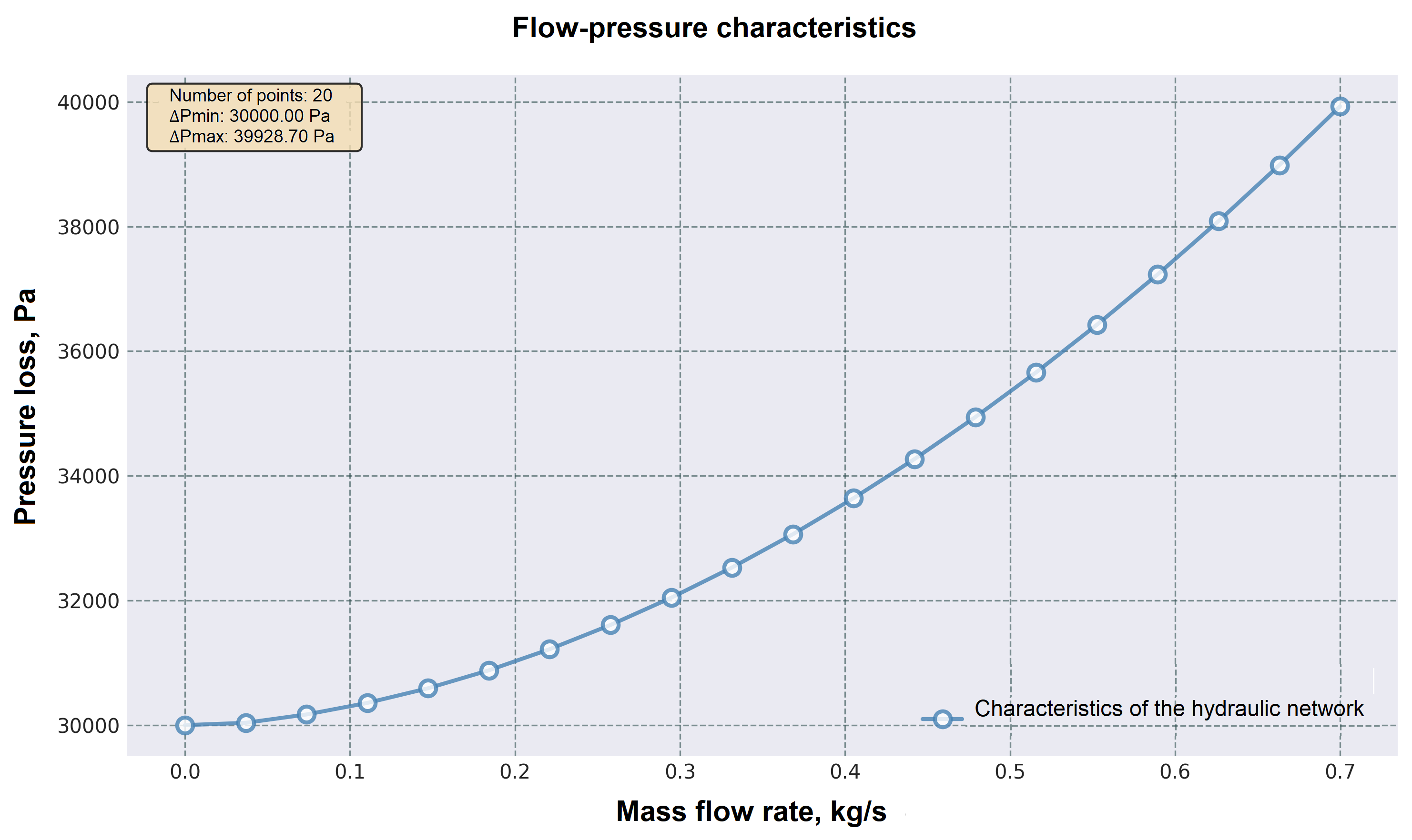
Fig. 9 FPC network#
6. Application of network characteristics#
The network characteristics are the starting point for selecting pumping equipment for the system being designed. Based on them, you can select the necessary pump to provide the required flow and verify its operating point.
As an example, let’s consider the Wilo Star-RS 25/4 pump for operation in a simulated network. Its FPC is shown in Fig. 10 [1]:
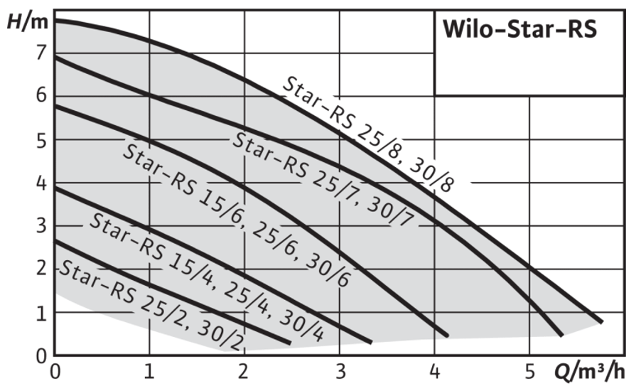
Fig. 10 WiloStar FPC series pumps#
We will take a number of points from the existing curve (in the range of interest to us) to add the curve to the graph of the FPC network (table 6):
Table 6 - Wilo Star-RS 25/4 FPC points
Consumption, m\(^3\)/h |
Consumption, kg/s |
Head, m |
Head, Pa |
|---|---|---|---|
0 |
0 |
||
1 |
|||
Let’s add the pump’s FPC to the graph. The code, with the necessary modifications, is presented below.
Visualization of the FPC for the pump and network
# Данные для выбранного насоса Wilo Star-RS 25/4
pump_df = pd.DataFrame({
    'massFlowRate': [0.0, 0.0693, 0.1386, 0.2079, 0.2772, 0.3465, 0.3881],
    'pressureDrop': [38182.5, 36028.6, 33776.8, 31525.0, 29077.4, 26434.0, 24867.6]
})

# Импортируем и устанавливаем необходимые библиотеки для визуализации
import matplotlib.pyplot as plt
await piplite.install("seaborn")
import seaborn as sns

def plot_pressure_drop_curve(results_df, pump_df, figsize=(10, 6)):
    """
    Создает график зависимости потерь давления от массового расхода.

    Parameters:
    -----------
    results_df : pd.DataFrame
        DataFrame с колонками 'massFlowRate' и 'pressureDrop' для характеристики сети
    pump_df: pd.DataFrame
        DataFrame с колонками 'massFlowRate' и 'pressureDrop' для характеристики насоса
    figsize : tuple
        Размер графика в дюймах (ширина, высота)
    """

    # Настройка стиля графика
    plt.style.use('seaborn-v0_8-dark')

    # Создаем фигуру и оси с указанным размером
    fig, ax = plt.subplots(figsize=figsize, dpi=100)

    # Фильтруем данные, исключая NaN значения для чистоты графика
    clean_data = results_df.dropna(subset=['pressureDrop'])
    #Данные для насоса
    clean_pump_data = pump_df.dropna(subset=['pressureDrop'])
    # Проверяем, есть ли данные для отображения
    if len(clean_data) == 0:
        print("Нет данных для построения графика (все значения NaN)")
        return

    # Создаем основной график - линию с маркерами
    # Используем маркеры 'o' для точек и линию для соединения
    ax.plot(clean_data['massFlowRate'],
            clean_data['pressureDrop'],
            marker='o',                # Маркеры в виде кружков
            markersize=8,              # Размер маркеров
            linewidth=2,               # Толщина линии
            color='steelblue',         # Цвет линии
            alpha=0.8,                 # Прозрачность
            label='Характеристика гидравлической сети',   # Метка для легенды
            markerfacecolor='white',   # Заливка маркеров
            markeredgewidth=2)         # Толщина обводки маркеров
    # График РНХ насоса
    ax.plot(clean_pump_data['massFlowRate'],
            clean_pump_data['pressureDrop'],
            marker='o',                # Маркеры в виде кружков
            markersize=8,              # Размер маркеров
            linewidth=2,               # Толщина линии
            color='#e63946',            # Цвет линии
            alpha=0.8,                 # Прозрачность
            label='Характеристика насоса',   # Метка для легенды
            markerfacecolor='white',   # Заливка маркеров
            markeredgewidth=2)         # Толщина обводки маркеров

    # Добавляем маркеры для выделения отдельных точек
    # Полезно при малом количестве точек
    if len(clean_data) <= 10:
        # Добавляем подписи значений над точками
        for idx, row in clean_data.iterrows():
            ax.annotate(f"{row['pressureDrop']:.2f}",
                       xy=(row['massFlowRate'], row['pressureDrop']),
                       xytext=(0, 10),  # Смещение текста относительно точки
                       textcoords='offset points',  # Координаты смещения в пунктах
                       ha='center',  # Горизонтальное выравнивание
                       fontsize=9,
                       color='darkslategray')

    # Настройка осей графика
    ax.set_xlabel('Массовый расход, кг/с',
                  fontsize=12,
                  fontweight='bold',
                  labelpad=10)  # Отступ подписи от оси

    ax.set_ylabel('Потери давления, Па',
                  fontsize=12,
                  fontweight='bold',
                  labelpad=10)  # Отступ подписи от оси

    # Заголовок графика
    ax.set_title('Расходно-напорная характеристика',
                 fontsize=14,
                 fontweight='bold',
                 pad=20)  # Отступ заголовка

    # Добавляем сетку
    ax.grid(True, which='both', linestyle='--', color='#2F4F4F', alpha=0.6)

    # Настраиваем пределы осей с небольшим запасом
    x_min, x_max = clean_data['massFlowRate'].min(), clean_data['massFlowRate'].max()
    y_min, y_max = clean_data['pressureDrop'].min(), clean_data['pressureDrop'].max()

    # Добавляем 5% запаса по осям
    x_padding = (x_max - x_min) * 0.05
    y_padding = (y_max - y_min) * 0.05

    ax.set_xlim(x_min - x_padding, x_max + x_padding)
    ax.set_ylim(y_min - 12 * y_padding, y_max + y_padding)

    # Добавляем легенду с настройками позиционирования
    ax.legend(loc='lower right',
          bbox_to_anchor=(1.0, 0.012),
          fontsize=10,
          framealpha=0.9,
          facecolor='#2F4F4F',
          edgecolor='white')

    # Добавляем статистическую информацию в угол графика
    stats_text = f"Количество точек: {len(clean_data)}\n" \
                 f"ΔP мин: {clean_data['pressureDrop'].min():.2f} Па\n" \
                 f"ΔP макс: {clean_data['pressureDrop'].max():.2f} Па"

    ax.text(0.02, 0.98, stats_text,
            transform=ax.transAxes,  # Используем относительные координаты
            verticalalignment='top',
            bbox=dict(boxstyle='round', facecolor='wheat', alpha=0.8),
            fontsize=9)

    # Настраиваем внешний вид графика
    # Убираем лишние отступы
    plt.tight_layout()

    # Отображаем график
    plt.show()

    # Возвращаем объекты фигуры и осей для возможной дальнейшей настройки
    return fig, ax

# Создаем график
fig, ax = plot_pressure_drop_curve(results_df, pump_df)
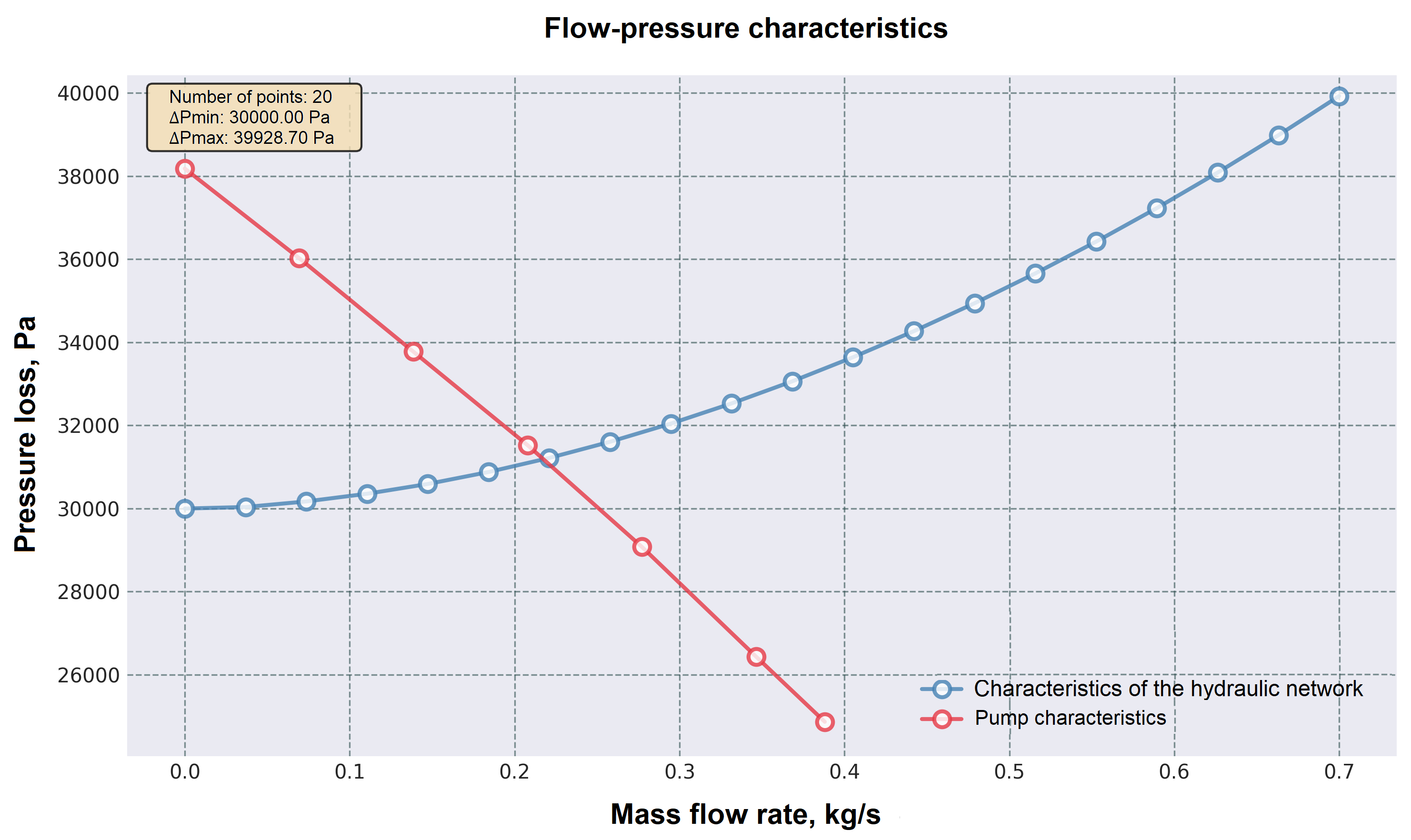
Fig. 11 Pump and network characteristics graphs#
As a result of executing the code, you get the FPC of the network and the pump on one graph (see Fig. 11 above), which allows you to visually determine the operating point of the pump in the simulated network. According to the obtained graphs, the operating point of the pump corresponds to a flow rate of about 0.22 [kg/s].
6.1. Determining the operating point of a pump in a mathematical model#
Let’s go to the model and add a Tabulated pump (TL) block between the filter and pipeline 2 and a Flow Rate Sensor (TL) block (use the pump as the associated block). Then delete the block Ideal flow rate source (TL), Fig. 12:
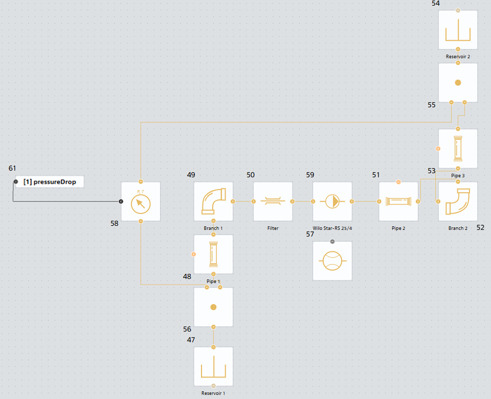
Fig. 12 Model with pump#
Fill in the pump properties according to Table 7. The properties are set based on the pump curve defined earlier.
Table 7 - Properties of the Tabulated pump (TL) block
Property/Custom block name |
Wilo Star-RS 25/4 |
|---|---|
Port area, m² |
|
Reference head vector, m |
|
Capacity vector, lpm |
Run the model for calculation and take readings from the flow sensor.
The flow rate value is 0.21875383 [kg/s], which corresponds to the previously constructed curves and the graphically determined operating point, Fig. 13:
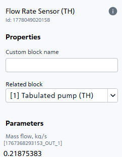
Fig. 13. Flow rate of the medium in the mathematical model#
7. Conclusions#
During the course of the tutorial, the methodology for constructing a FPC for a hydraulic network using SW REPEAT VISION was successfully mastered. The practical work allowed us to go through the full cycle of engineering analysis: from the creation and correct configuration of a calculation model, including tanks, pipelines and local resistances, to the automation of parametric calculations using the JupyterLite scripting environment to obtain an array of data. As a result, a network characteristic was constructed.
Thus, the mastered tools for constructing FPC in REPEAT VISION represent the basis for designing, analyzing and optimizing thermal hydraulic systems, ensuring a well-founded selection of pumping equipment and forecasting its efficient operation within a specific network.