Thermal conductivity in a flat wall

This tutorial describes simple steps to set up a circuit to solve a heat transfer problem.

The following task is considered as part of the tutorial:

The temperature of inner and outer surfaces of the window glass with a thickness of 5 [mm] is 15 and 5[℃] accordingly. What is the heat loss through a window of size 1×3 [m]? Thermal conductivity of glass is 1.4 [W/(m∙K)].

1.  Create and set up a project

First, it is necessary to create a new project and give it a name, for example, Thermal Conductivity in a Flat Wall.

The next step is to set the Simulation Time by assigning a value of 1 second to the corresponding project parameter, Fig. 1:

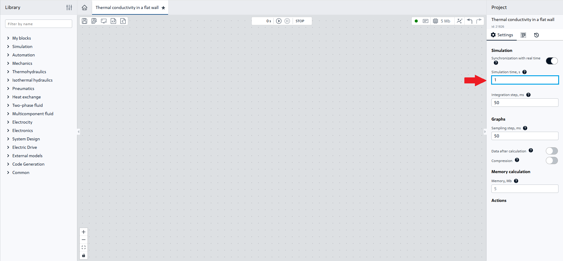
Fig. 1 Setting the simulation time

Start the basic steps to create a thermal model by opening the Heat exchange library.

2.  Create temperature sources

As part of task, temperatures on the inner and outer surfaces of the glass are set. In order to simulate these boundary conditions, use the Temperature source block and move it to the workspace, Fig. 2:

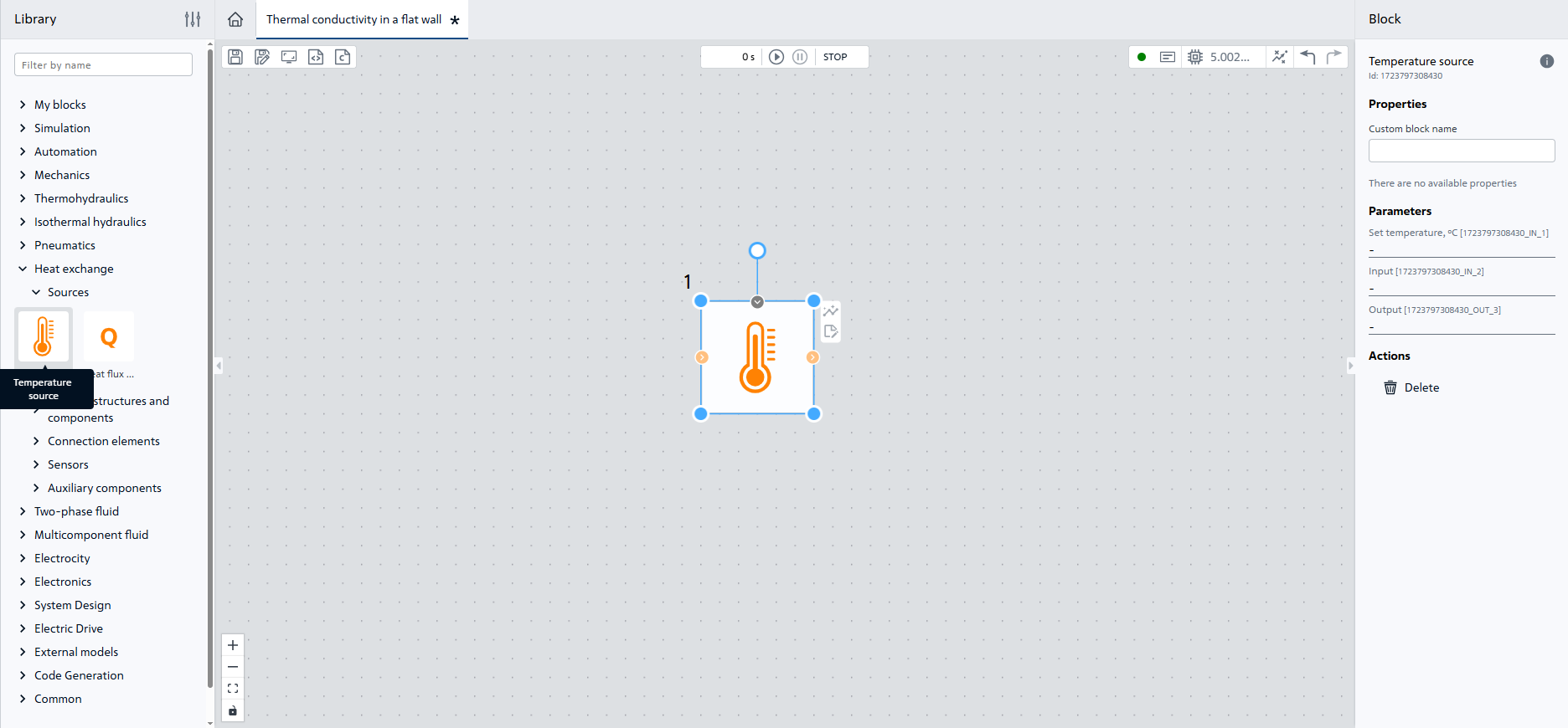
Fig. 2 Adding the Temperature source block

This block is a controlled source, i.e. a signal shall be sent to the upper port of the block to set the temperature value.

As part of the task, temperatures on glass surfaces remain constant, so use the Constant block, add it to the workspace, assign a constant value of 15 in the properties and connect the blocks to each other, Fig. 3:

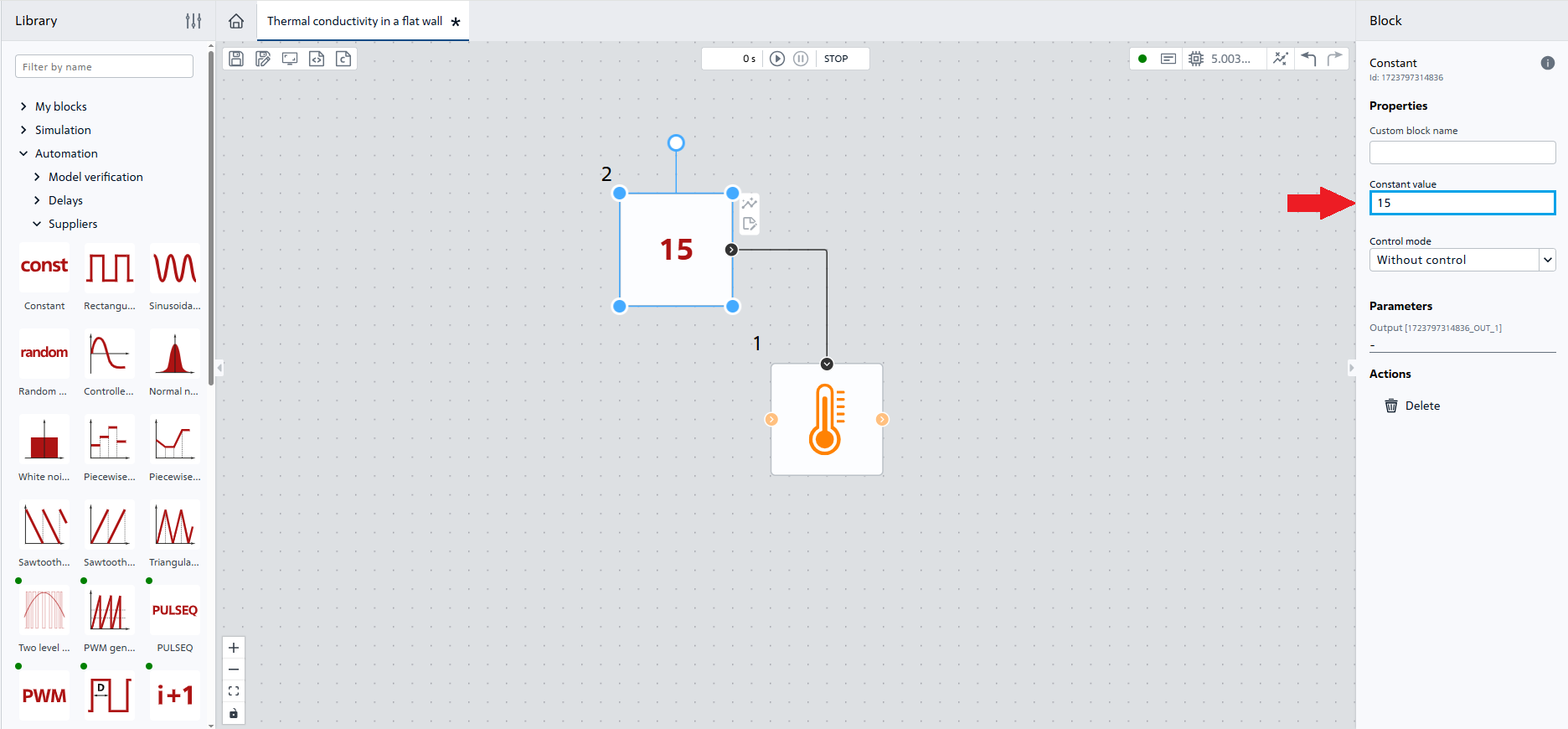
Fig. 3 Adding and connecting the Constant block

Important

The signal can be constant (using a Constant block) and variable (for example, a Sinusoidal wave generator, Piecewise constant function, etc.).

Next, it is necessary to add a similar group of blocks to the workspace to set the boundary condition on the outer surface. Add this group of blocks by holding Ctrl and clicking on each block and links between them to select them. Then it is necessary to press Ctrl+C, Ctrl+V buttons to copy a group of blocks and links between them, and paste them to the canvas. Then it is necessary to assign the Constant value - 5 property for the new Constant block, Fig. 4:

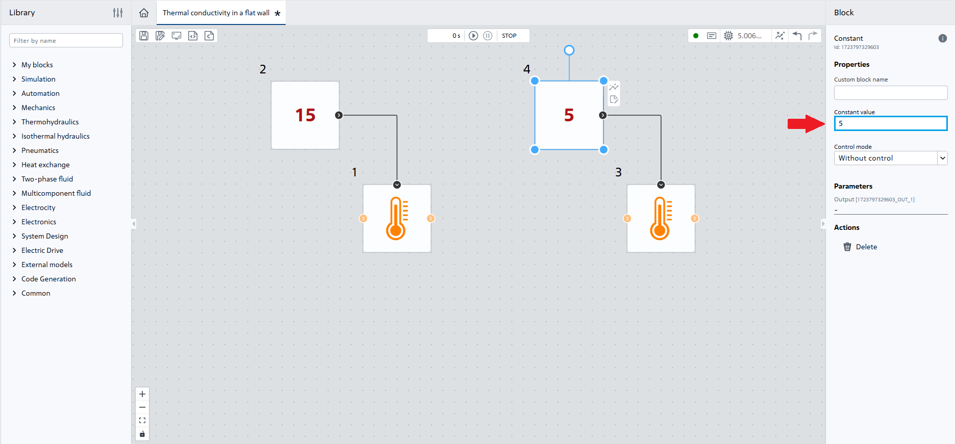
Fig. 4 Adding a similar group of blocks

Boundary conditions for the problem have been established, so move on to simulation of the flat wall.

3.  Wall creation

In order to simulate heat transfer in a flat wall, use Conductive heat transfer block. Move the block to the workspace and change the values of block properties to the following, according to the problem condition:

1. Surface area: 3.0 [m\(^2\)];

2. Wall thickness: 0.005 [m];

3. Thermal conductivity: 1.4 [W/(m∙ᵒC)].

Important

In REPEAT VISION decimal numbers are separated by a dot.

Next, connect the blocks as shown in the Fig. 5 below:

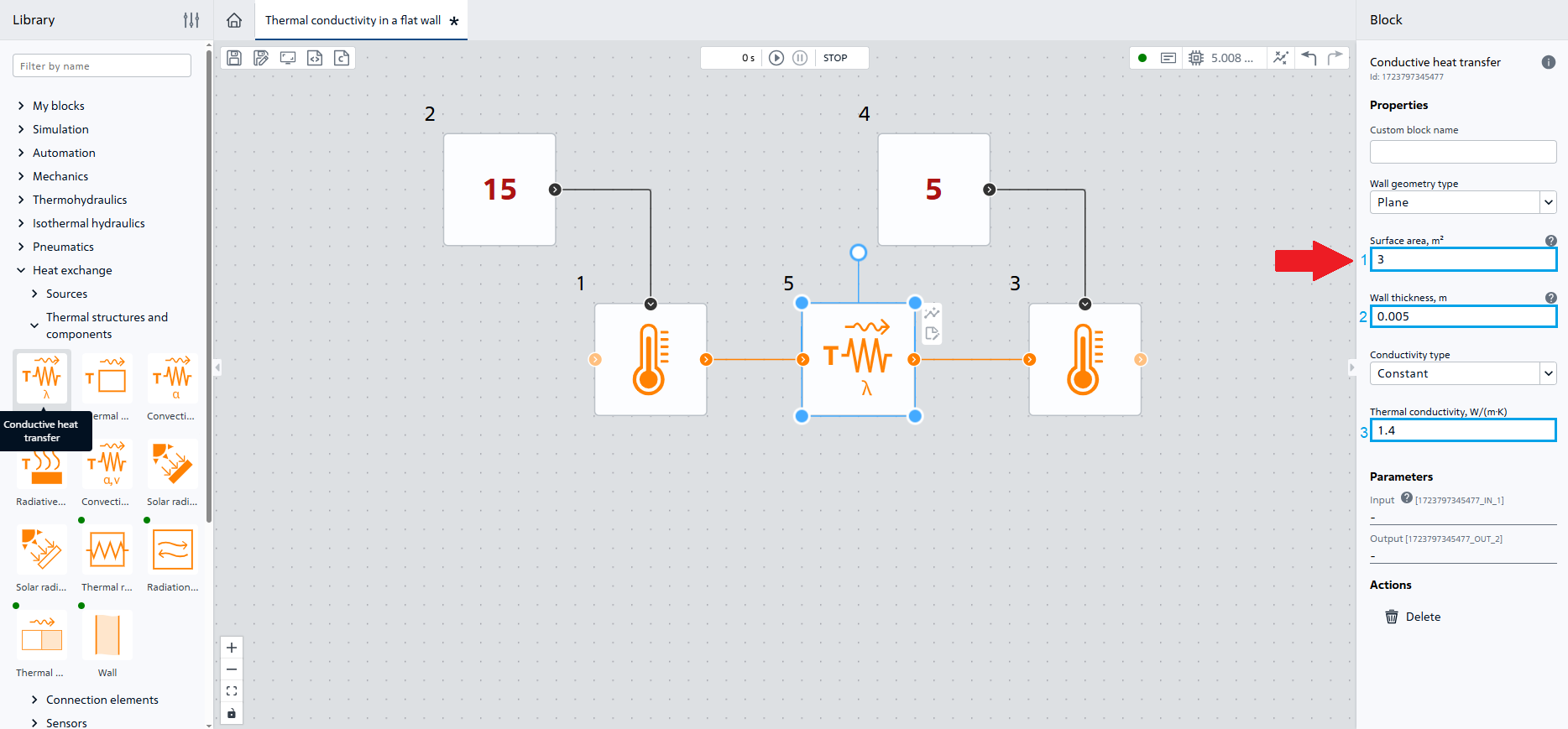
Fig. 5 Connecting blocks

4.  Display of calculation results

In order to remove the heat flux through the wall, add a Meter block.

From the drop-down list:

1. Select Conductive heat transfer 1 for the Block property;

2. For property Parameter - Heat flow, [W].

Save the project, Fig. 6:

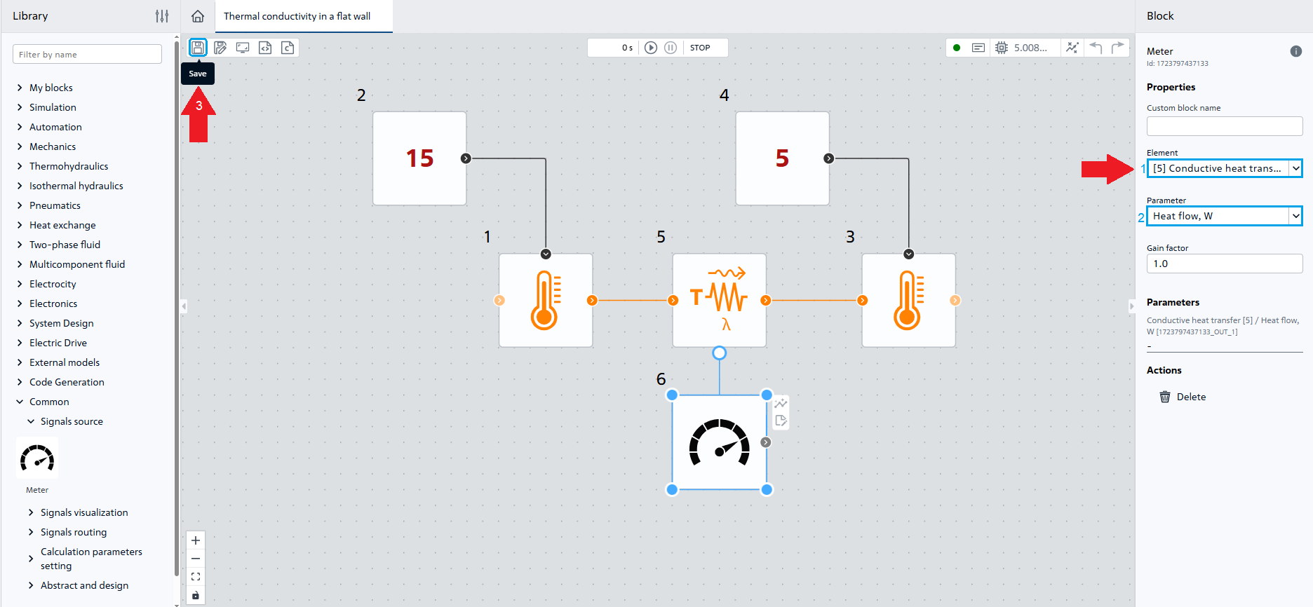
Fig. 6 Saving the project

The thermal model is ready for calculation.

5.  Start calculation

Start the calculation with “Start Simulation” button

The calculation shall be successfully completed with the following message:

Modeling stopped on the solver side due to modeling time limit exceeded.

6.  Analysis of calculation results

After successful completion of the calculation, the heat flow at the end of simulation time will be indicated in the Meter block. The heat flow value shall be 8400 [W], Fig. 7:

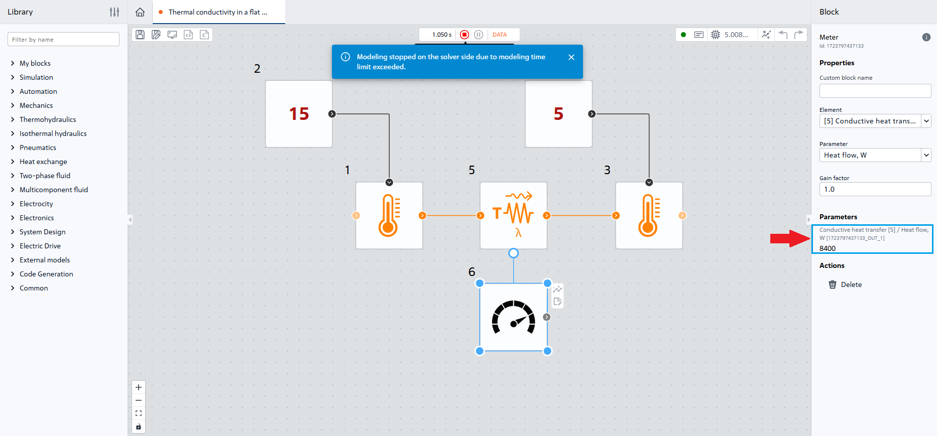
Fig. 7 Obtaining the heat flow value

7.  Conclusions

As a result of this tutorial, you have gained basic knowledge for solving heat exchange problems. You have learned:

• Create temperature boundary conditions for heat exchange models using the Temperature source block;

• Define heat flux values in a flat wall with specified properties and geometry;

• Read the heat flux values using the Meter block.