Short circuit in the power system

This tutorial describes simple steps to simulate a short circuit (SC) in a three-phase single-machine power system.

This tutorial deals with a problem in which SC is simulated in a power system with a nominal voltage of 220 [kV]. This energy area comprises three-phase voltage source, PTL and load. As a result of the calculation, it is required to determine the shock value of the current in phase A after the occurrence of SC.

1.  Project creation and setup

First you need to create a new project and give it a name, for example, SC in the power system.

In the next step, one needs to make the following settings (see Fig. 1 below):

Setup	Value
1 Synchronization with real time	Disable
2 Simulation time	0.1 [s]
3 Integration step	0.05 [ms]
4 Sampling step	0.05 [ms]

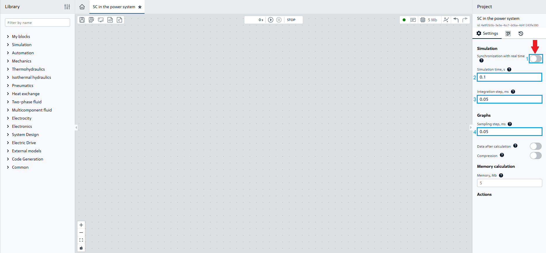
Fig. 1 Project setup

Note

Disable parameter to set the simulation time to < 1[s]

Important

In REPEAT VISION decimal numbers are specified through a period.

Let’s start the basic steps for creating a diagram by opening the library Electronics.

2.  Three-phase voltage source creation

Add block №1 of our diagram, for this purpose we will transfer it to the workspace block Three-phase voltage source.

Note

This block represents the equivalent of the power system that powers the area.

In the properties of block №1 specify (see Fig. 2 below):

Property	Value
1 Phase-to-phase RMS voltage	230000 [V]
2 Source resistance	1 [Ohm]
3 Source inductance	0.001 [H]

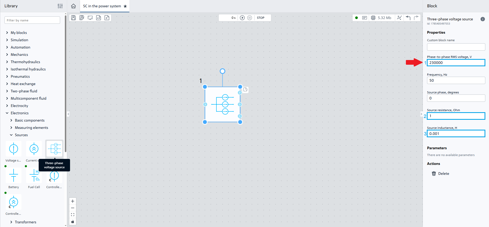
Fig. 2 Properties of block №1

3.  Creating PTL 220 [kV]

In order to simulate PTL 220 [kV], which is designed to transmit electric energy and power to the load, let’s transfer block №2 Three-phase series RLC branch to the workspace, set the following properties and then place and connect the blocks in accordance with the fig. 3 below:

Property	Value
1 Branch type	RL
2 Phase resistance	18.15 [Ohm]
3 Phase inductance	0.208 [H]

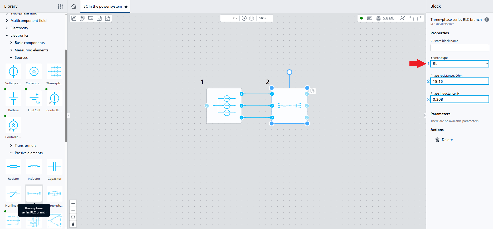
Fig. 3 Properties of block №2 and its connection to the diagram

Note

The given parameters are calculated based on the design parameters of the AC 240/32 wire [1] with the PTL 150 [km] length.

4.  Adding assemblies

For the possibility of connecting the zero potential of the voltage source and simulation SC, add block №3 at the end of the line Node , for this purpose one needs to transfer the block №3 of the same name to the workspace. We need 5 of these blocks, so let’s use one of the ways to add them:

Classic transfer of the block from the library to the left

For this purpose, drag block №4 to the workspace.

Copying the block located in the workspace

For this purpose, one shall:

1. Select block №3 with the LMB;

2. Press a combination of buttons CTRL+C and CTRL+V.

• For blocks №3-6, which get connected to blocks №1 and №2 Three-phase voltage source and Three-phase series RLC branch, specify the value of the Number of output ports property - 2.

• For block №7 necessary to create SC, let’s set the value of the Number of input ports property to 3 and turn it counterclockwise by 90⁰:

Place and connect the blocks in accordance with the Fig. 4 :

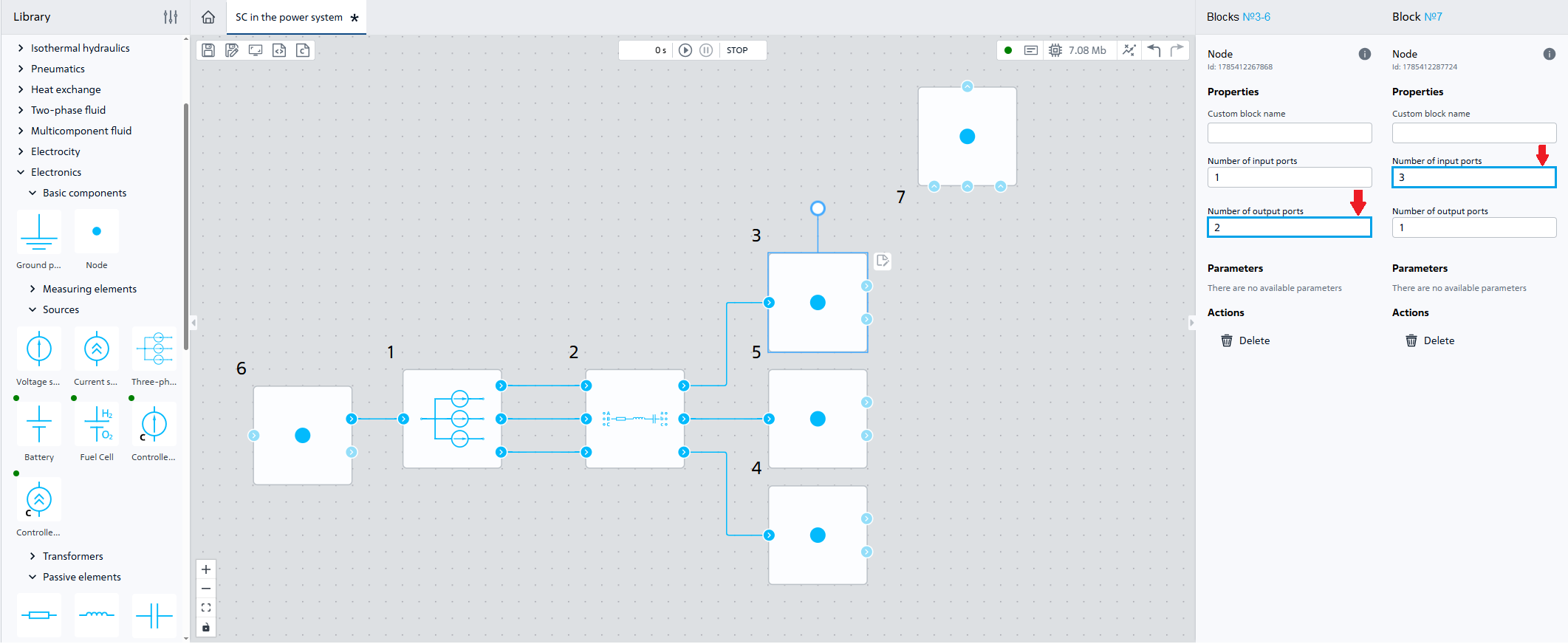
Fig. 4 Properties of blocks №3-7 and its connection to the diagram

5.  Load creation

For setting the load with the «star» connection circuit st voltage of 220 [kW] add block №8 Three-phase series RLC wye load . Transfer block №8 of the same name to the workspace, in its properties specify:

Property	Value
1 Branch type	RL
2 Nominal phase-to-phase voltage	220e3 [V]
3 Three-phase active power	40e6 [W]
4 Inductive power	30e6 [VAr]

Then place and connect the block in accordance with the Fig. 5:

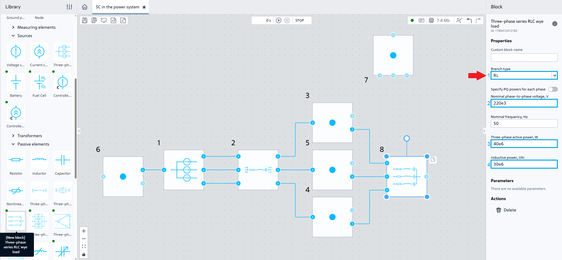
Fig. 5 Properties of block №8 and its connection to the diagram

6.  Adding zero potential

Let’s transfer of the same name block №9Ground potential to the workspace for grounding the zero outputs of the voltage source and load at the voltage of 220 [kW], setting single-phase SC.

We need three such blocks, for this we will use one of the methods described above.

Connect them to the outputs of block №6, block №8 and block №7. Place and connect the blocks in accordance with the Fig. 6:

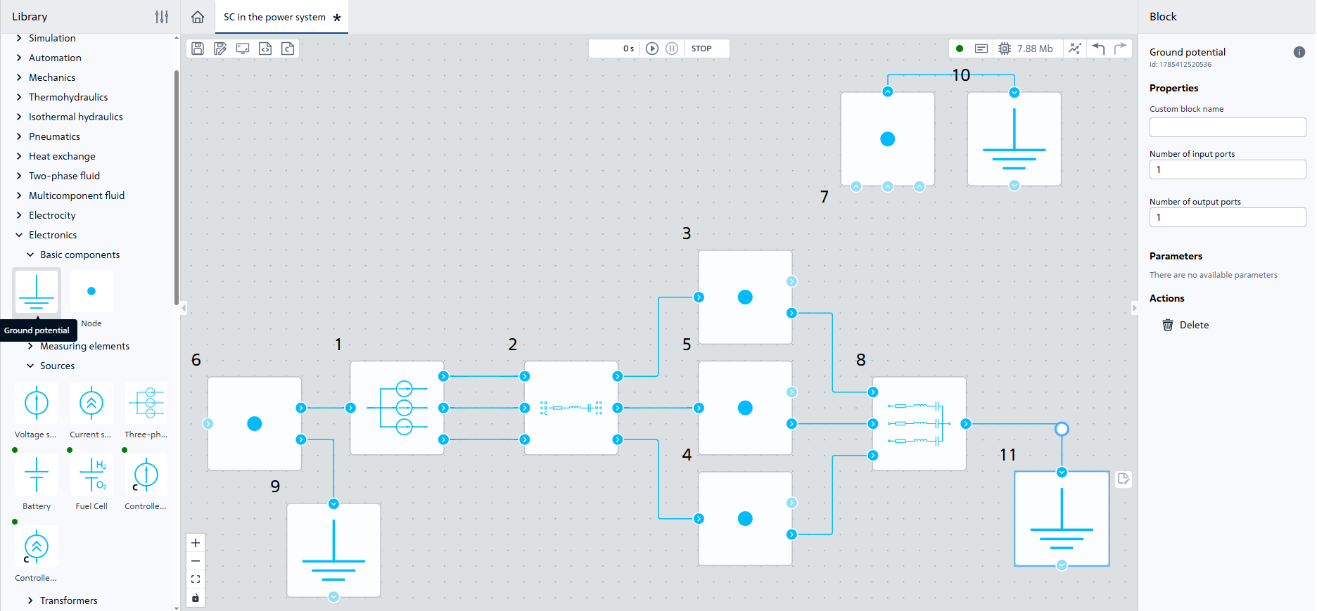
Fig. 6 Connection of blocks №9-11

7.  Adding sensors

In order to display the voltage signals of phases of load and current, let’s add blocks №12-17 Meter to the workspace in the line.

• In the properties of blocks №12-14 specify (see Fig. 7 below):

block №12

1. _Element - Three-phase series RLC branch;

2. Parameter - Phase current of phase A, A.

block №13

1. _Element - Three-phase series RLC branch;

2. Parameter - Phase current of phase B, A.

block №14

1. _Element - Three-phase series RLC branch;

2. Parameter - Phase current of phase C, A.

• In the properties of blocks №15-17 specify:

block №15

1. Element - Three-phase series RLC wye load;

2. Parameter - Phase-to-neutral voltage of phase A, V;

3. Gain factor - 1e-3.

block №16

1. Element - Three-phase series RLC wye load;

2. Parameter - Phase-to-neutral voltage of phase B, V;

3. Gain factor - 1e-3.

block №17

1. Element - Three-phase series RLC wye load;

2. Parameter - Phase-to-neutral voltage of phase C, V;

3. Gain factor - 1e-3.

Note

Setting gain factor 1e-3 will produce a voltage in [kV] on the charts, making the results easier to read and faster to analyze.

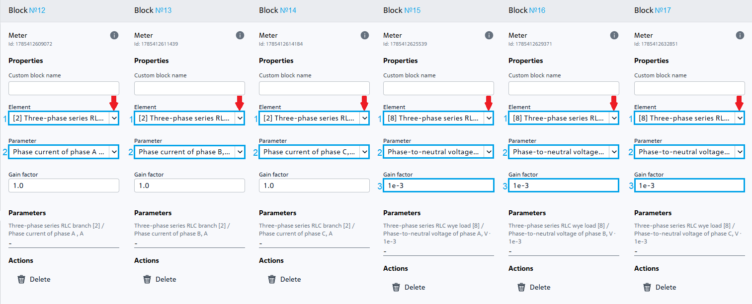
Fig. 7 Properties of blocks №12-17

Place the blocks in accordance with the Fig. 8:

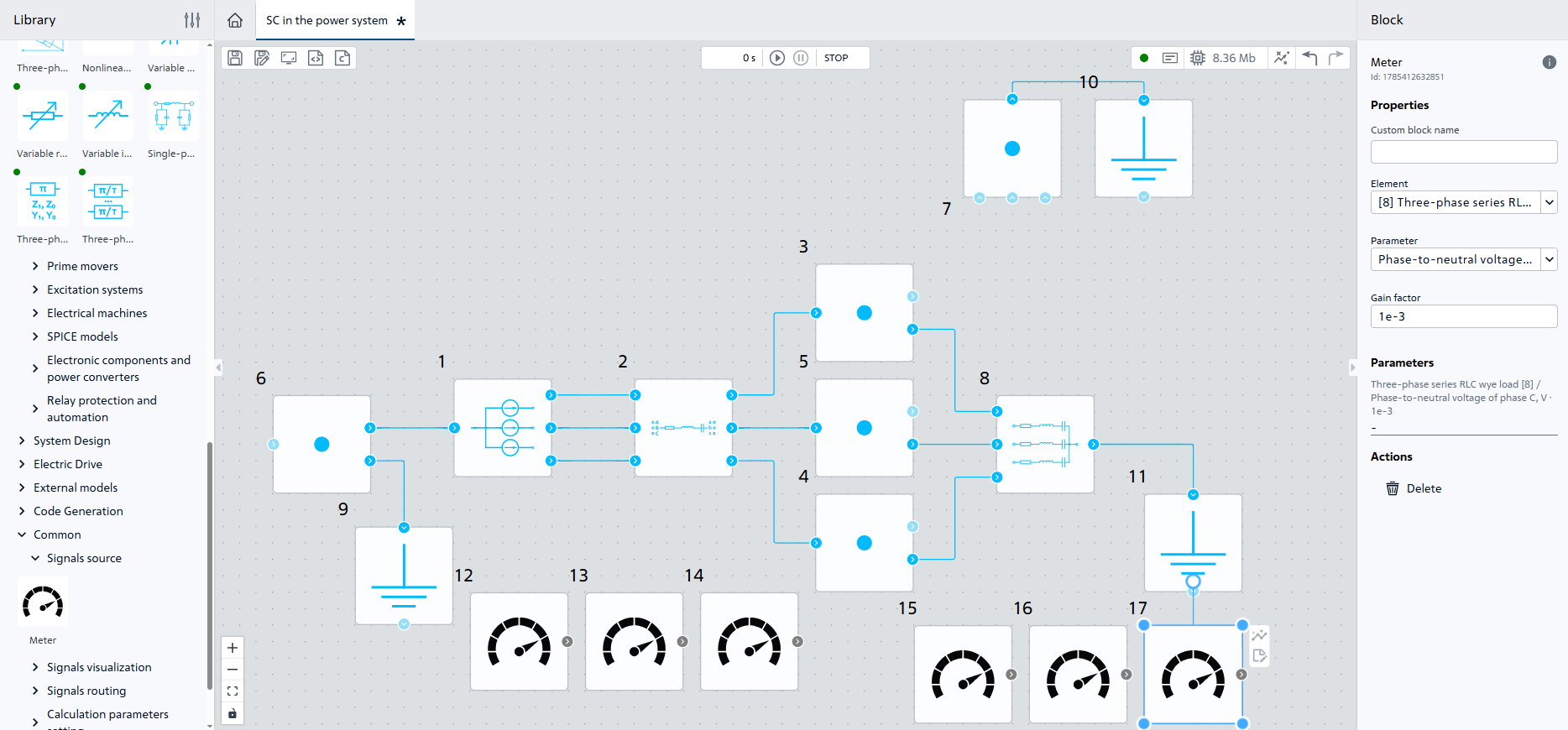
Fig. 8 Connection of sensors

8.  Let’s add the charts for visualization

1. Go to the Visualization tab (see Fig. 9 below);

2. Add two charts by double clicking on the button Add located in the right lower corner.

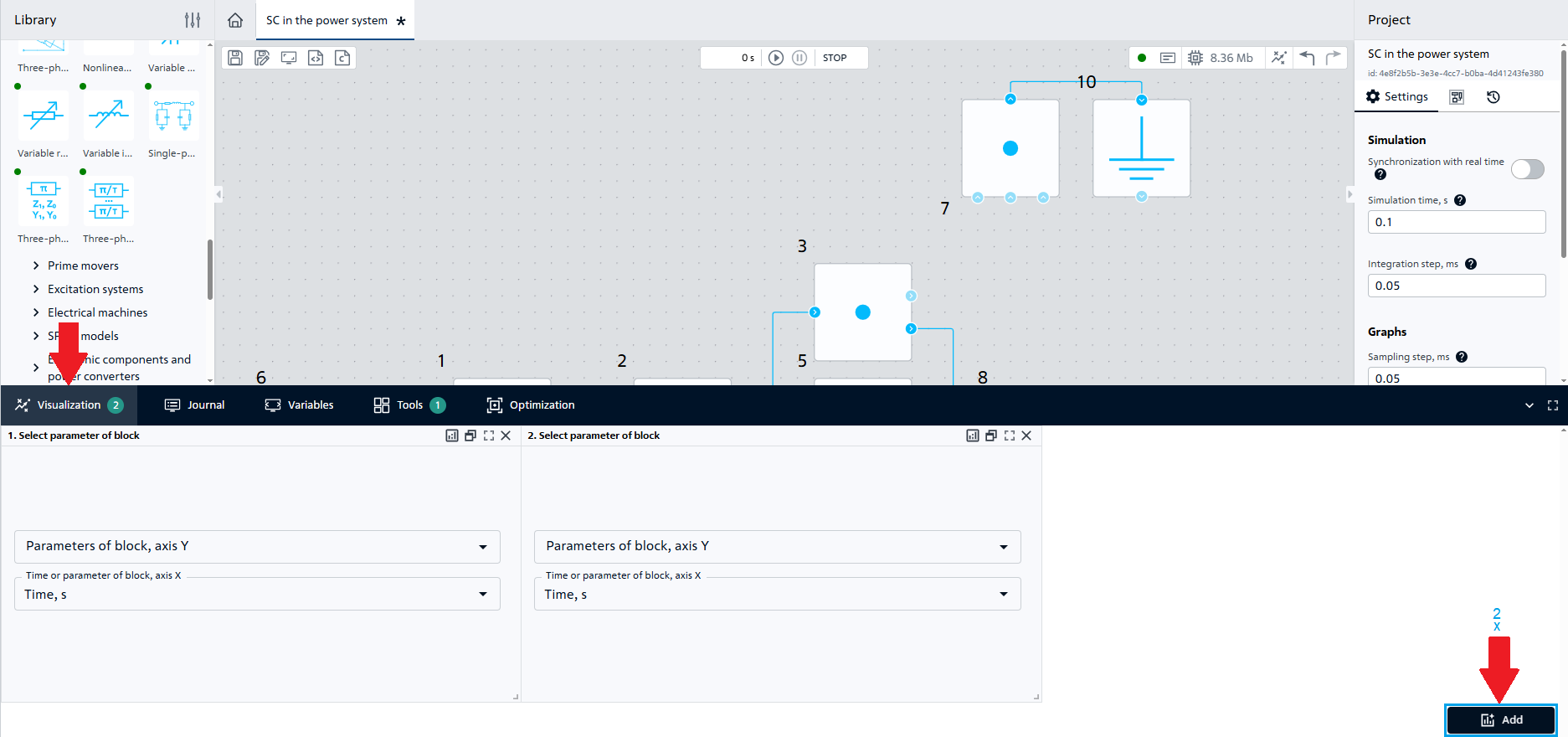
Fig. 9 Visualization

Then perform four steps for each chart to be added (see Fig. 10 below):

1. Add one chart to output signal of units №12-14;

2. Add second chart to output signal of blocks №15-17.

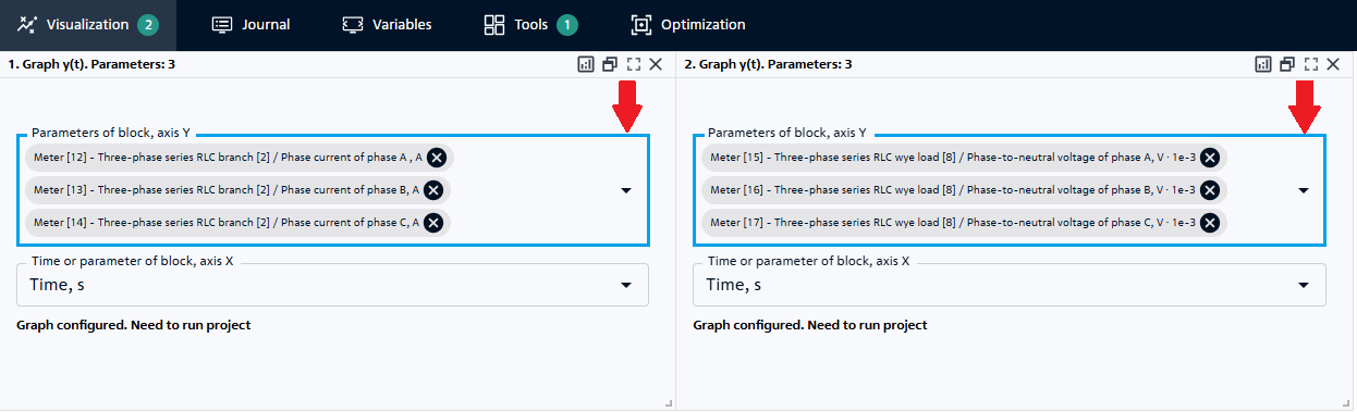
Fig. 10 Adding charts

9.  Simulation of single-phase SC

It is necessary to add the following blocks to simulate single-phase SC:

• block №18 Ideal switch for connection of current-carrying parts with the ground (in case of inter-phase SC – with each other);

• block №19 Piecewise constant function for control of block.

Let’s turn off the Snubber circuit property for block #18 (see Fig. 11 below):

Note

By changing the resistance of the key in the closed state, one can change the resistance in the point of SC, which will affect the value of current and voltage at SC.

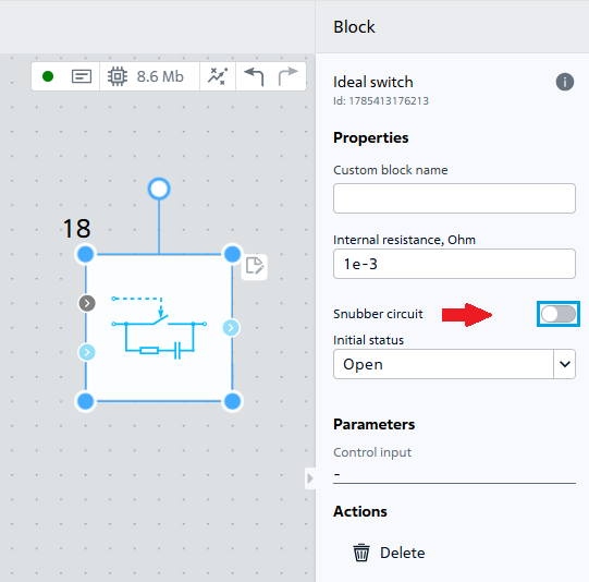
Fig. 11 Properties of block №18

Specify the following properties for block №19 (see Fig 12 below):

Property	Value
1 Vector of time arguments	0; 0.04 [s]
2 Vector of function values	0; 1
3 Periodicity	off

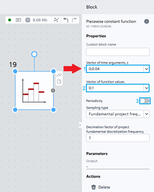
Fig. 12 Properties of block №19

Place and connect block №18 and block №19 in accordance with the Fig. 13 for simulation of single-phase SC in phase A :

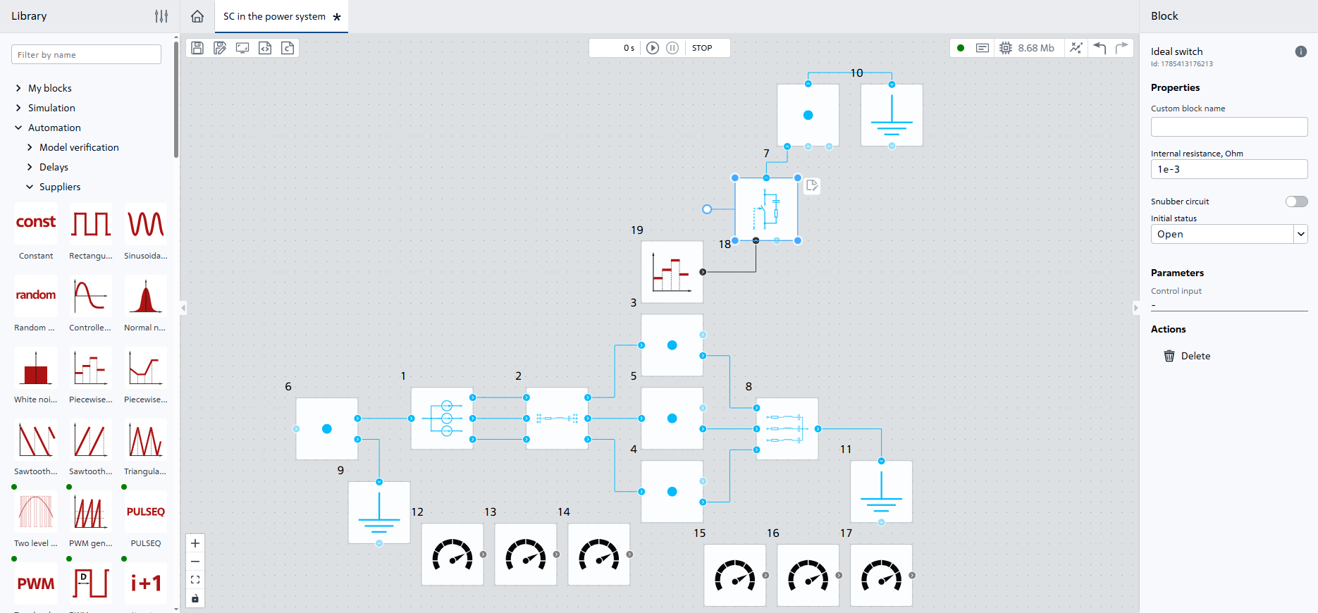
Fig. 13 Connection of blocks №18 and №19

Start calculation with the “Start simulation” button

The calculation should be successfully completed with the following message:

Modeling stopped on the solver side due to modeling time limit exceeded.

The previously created charts should now display the calculation results, which are shown in the Fig. 14, Fig. 15:

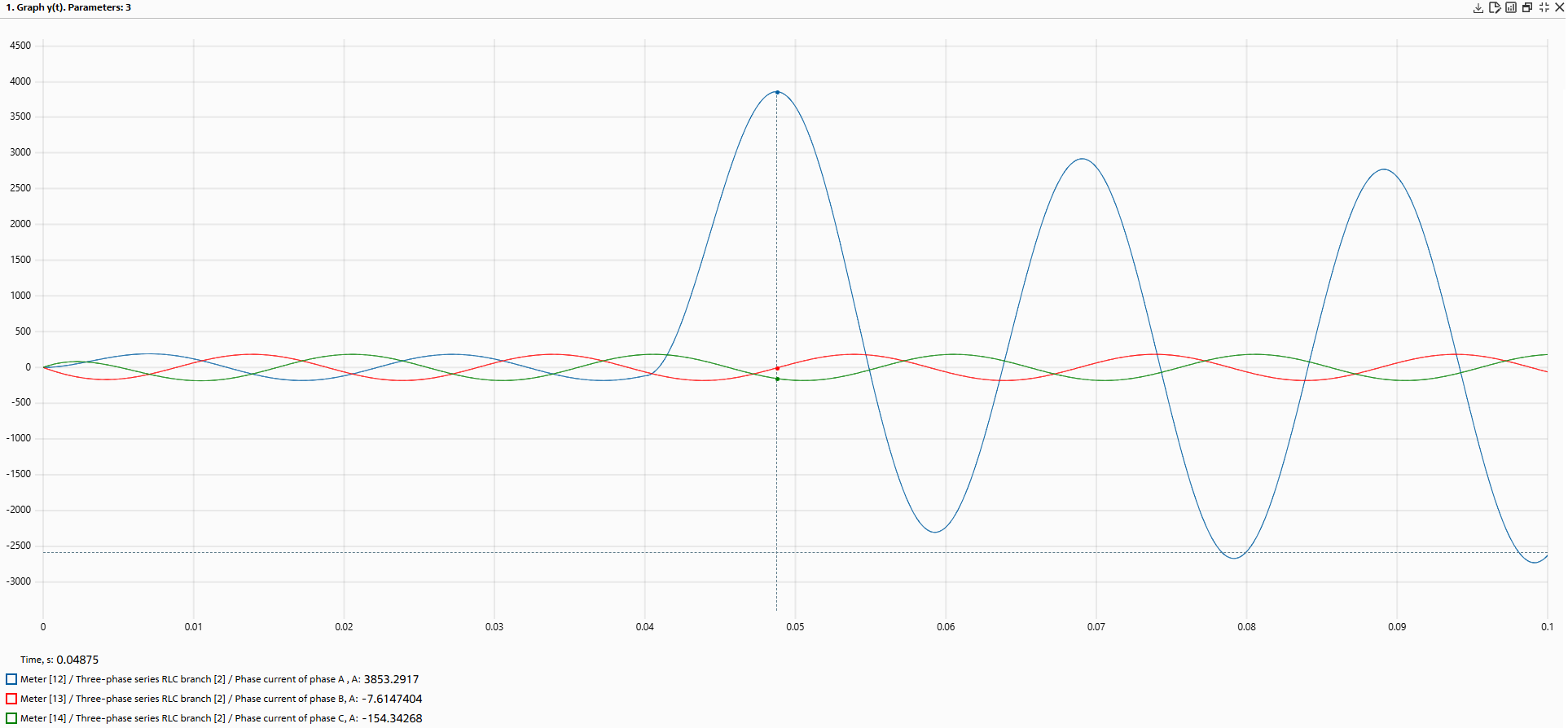
Fig. 14 Chart 1

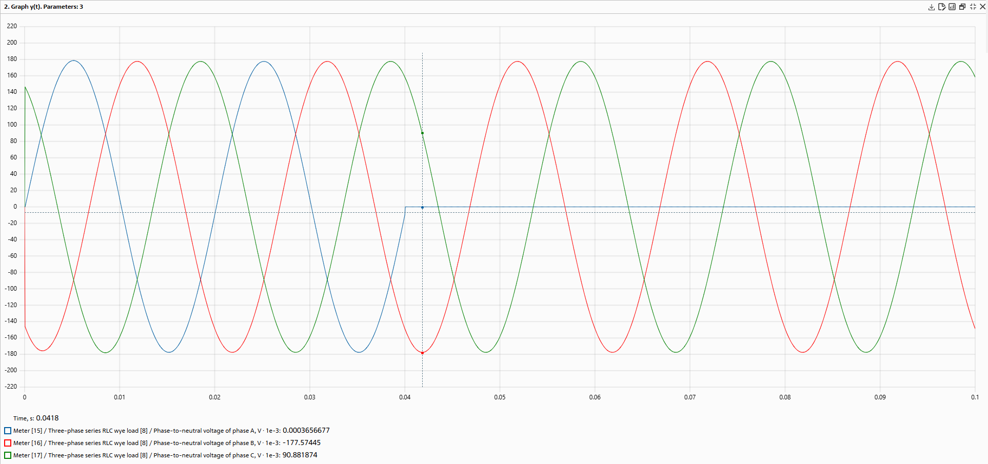
Fig. 15 Chart 2

Note

From the obtained oscillograms, we find the shock value of current in phase A (maximum instantaneous value) at single-phase SC - 3853 [A].

10.  Simulation of two-phase SC

In order to simulate a two-phase SC, it is necessary to:

1. Copy the previously created block №18 and block №19;

2. Connect “+” block №20 to output of block №4.

Hint

For ease of display, one can turn block №21 counterclockwise by 90⁰.

Hint

block №20 - this is a copy of block №18 and block №21 - this is a copy of block №19.

3. It is also necessary to disconnect the connection with the ground (remove the connection between block №7 and block №10) as in this type of CS phases close only to each other.

Place and connect blocks №20 and block №21 in accordance with the Fig. 16:

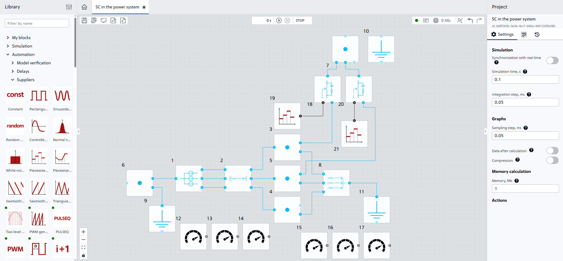
Fig. 16 Connection of blocks №20 and №21

Similar to the previous item, start simulation. The visualization will display charts of current and voltage in the network with two-phase SC, which are shown in the Fig. 17 and Fig. 18:

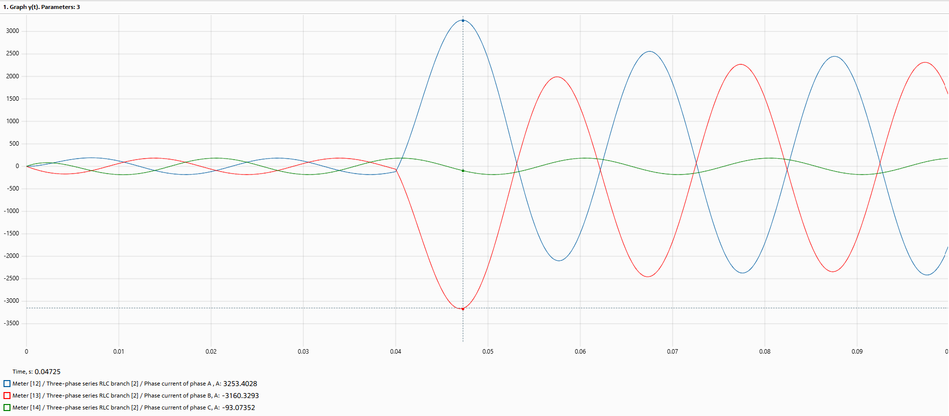
Fig. 17 Chart 1 (two-phase SC)

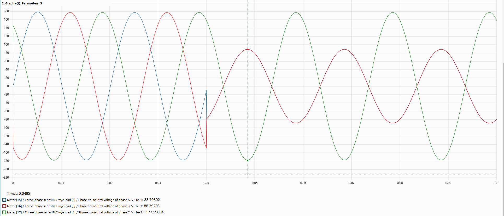
Fig. 18 Chart 2 (two-phase SC)

Note

From the obtained oscillograms, we find the value of shock current in phase A with two-phase SC – 3253 [А].

11.  Simulation of three-phase SC

In order to simulate a three-phase SC, it is necessary to:

1. Copy the previously created block №18 and block №19;

2. Connect “+” [block №22] (#title33) to output of block №5.

Hint

For ease of display, one can rotate block №23 counterclockwise by 90⁰.

Hint

block №22 - this is a copy of block №18 аnd block №23 - this is a copy of block №19.

Place and connect block №22 and block №23 in accordance with the Fig. 19:

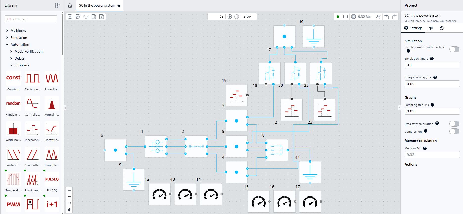
Fig. 19 Connection of blocks №22 and №23

Similar to step 9, start simulation. The visualization will display charts of current and voltage in the network with three-phase SC, which are shown in the Fig. 20 and Fig. 21:

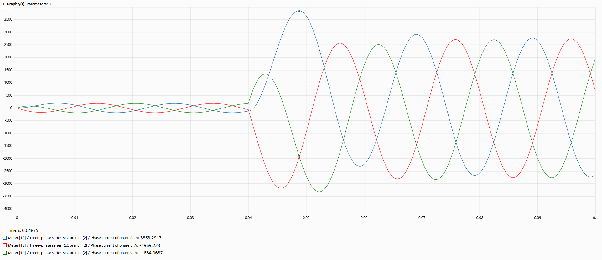
Fig. 20 Chart 1 (three-phase SC)

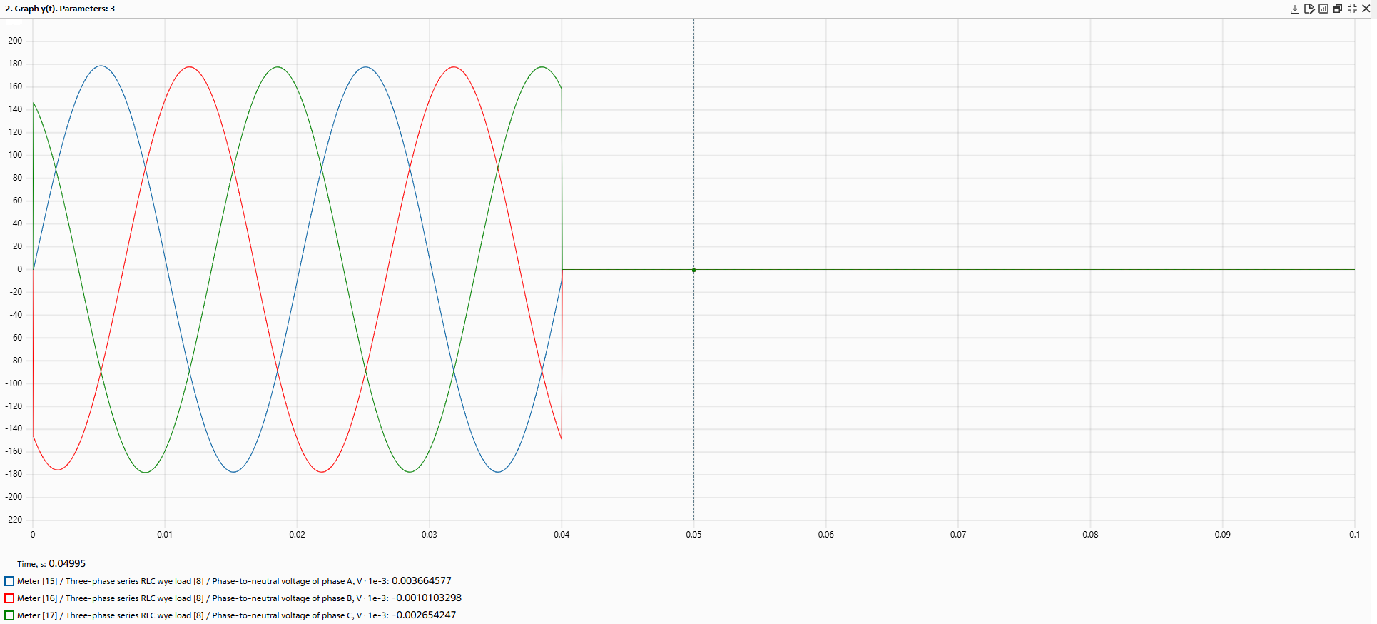
Fig. 21 Chart 2 (three-phase SC)

Note

From the obtained oscillograms, we find the value of the shock current in phase A with a three-phase SC – 3853 [А].

Hint

In order not to clutter the diagram, one can create a group with blocks for simulation SC. To do this, follow these steps:

1. Select blocks №7, №10, №18, №20, №22 and blocks №19, №21, №23 by holding down the SHIFT button, having previously connected blocks №7 and №10 to avoid creating unnecessary input and output ports, Fig. 22:

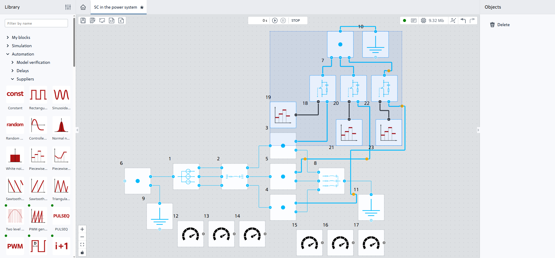
Fig. 22 Selection of blocks

2. Call the context menu using RMB and select Create group, Fig. 23:

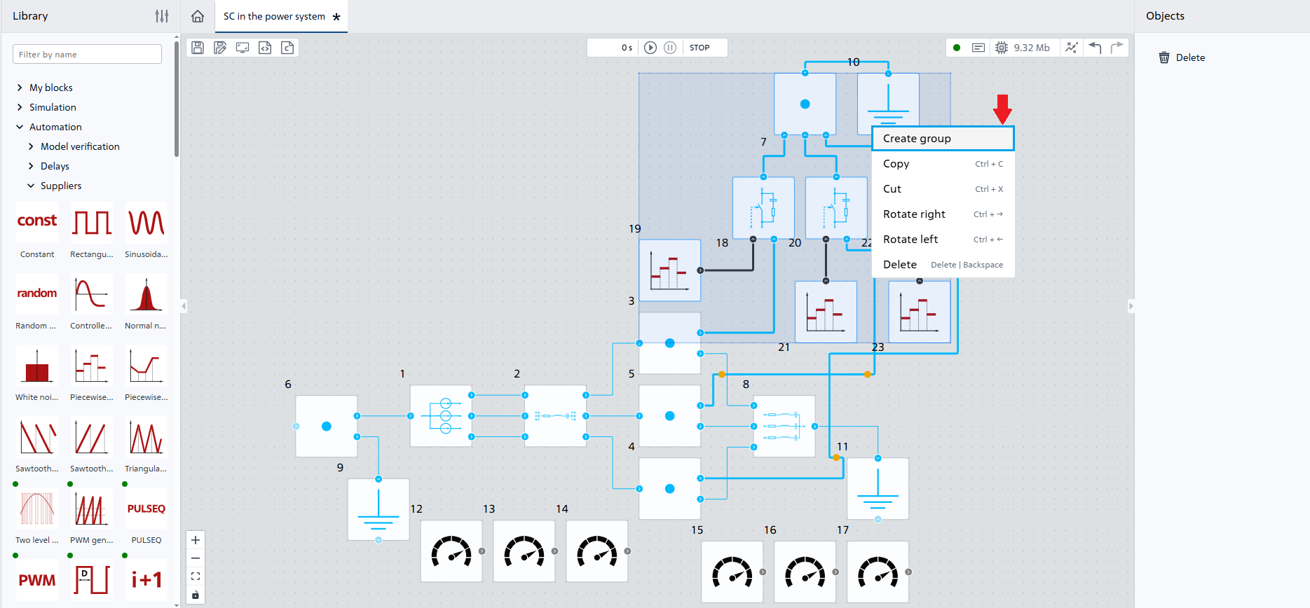
Fig. 23 Group creation

3. The resulting group can be turned for convenience, the name can be changed (by double-clicking on Group [7]) and the properties can also be added (for example, the parameters of block Piecewise constant function and the block Ideal switch), Fig. 24:

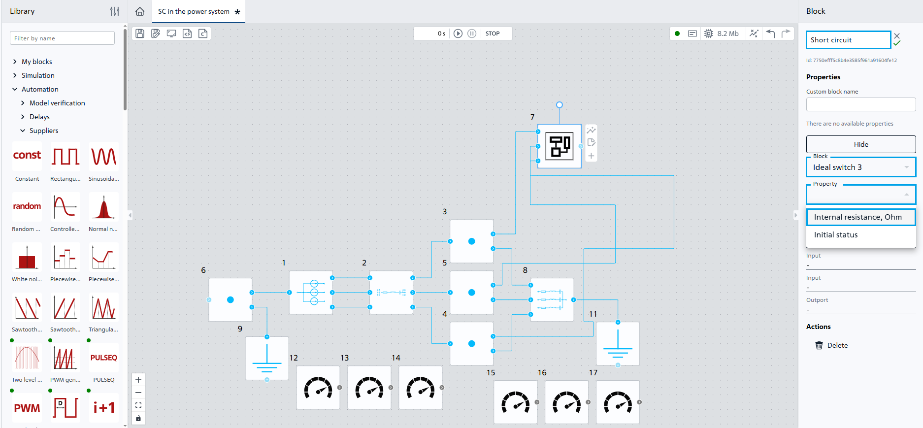
Fig. 24 Working with the group

4. One can also get inside the group by double-clicking LMB to remove/add blocks/links between blocks.

12.  Analysis of calculation results

The simulation results correspond to theoretical dependencies - with SC in the network, a multiple increase in current and a decrease in voltage in the damaged phase are observed. The shock current value for phase A with two-phase SC turned out to be less than with other types of SC, and the voltages of the damaged phases are equal to each other and not equal to 0, which also corresponds to the theory.

13.  Conclusions

As a result of this tutorial, you have gained basic knowledge for simulation of various types of SC in the power system. You have learned how to:

• set the block parameters Three-phase voltage source; Three-phase series RLC branch; Three-phase series RLC wye load; Ideal switch; Piecewise constant function;

• use block Piecewise constant function to control the block Ideal switch;

• use block Meter to display block signals;

• use blocks Ideal switch, Piecewise constant function, Node, Ground potential to simulate single-phase, two-phase and three-phase SC.

14.  Sources

---

[1]

B.N. Neklepayev, I.P. Kriuchkov Electric Part of Power Plants and Substations: Reference Materials for Course and Diploma Design: Study Guide for Universities. - 4th ed., revised and suppl. - M.: Energoatomizdat, 1989. – 608 p.: ill.