

Transient thermal conductivity in a steel rod#
In this tutorial, we will look at solving the transient heat transfer problem for thermal conductivity in a round steel rod:
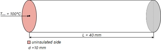
Fig. 1 Steel rod#
The following characteristics are accepted for steel 08Х18Н10Т:
Density - 7900 [kg/m3];
Temperature, ℃ |
Thermal conductivity, W/(m∙℃) |
|---|---|
100 |
16 |
200 |
18 |
300 |
19 |
Temperature, ℃ |
Specific thermal capacity, J/(kg∙℃) |
|---|---|
20 |
461 |
100 |
494 |
200 |
515 |
300 |
536 |
400 |
549 |
500 |
561 |
600 |
574 |
700 |
595 |
1. Project creation and setup#
Let’s create a new project and give it a name, for example, Transient thermal conductivity in a steel rod.
Then, since the process of achieving a steady state takes a long time, it is necessary to (see Fig. 2 below):
Set the
Synchronization with real timeparameter to off position;Set the
Simulation timeparameter value to 800 [s].
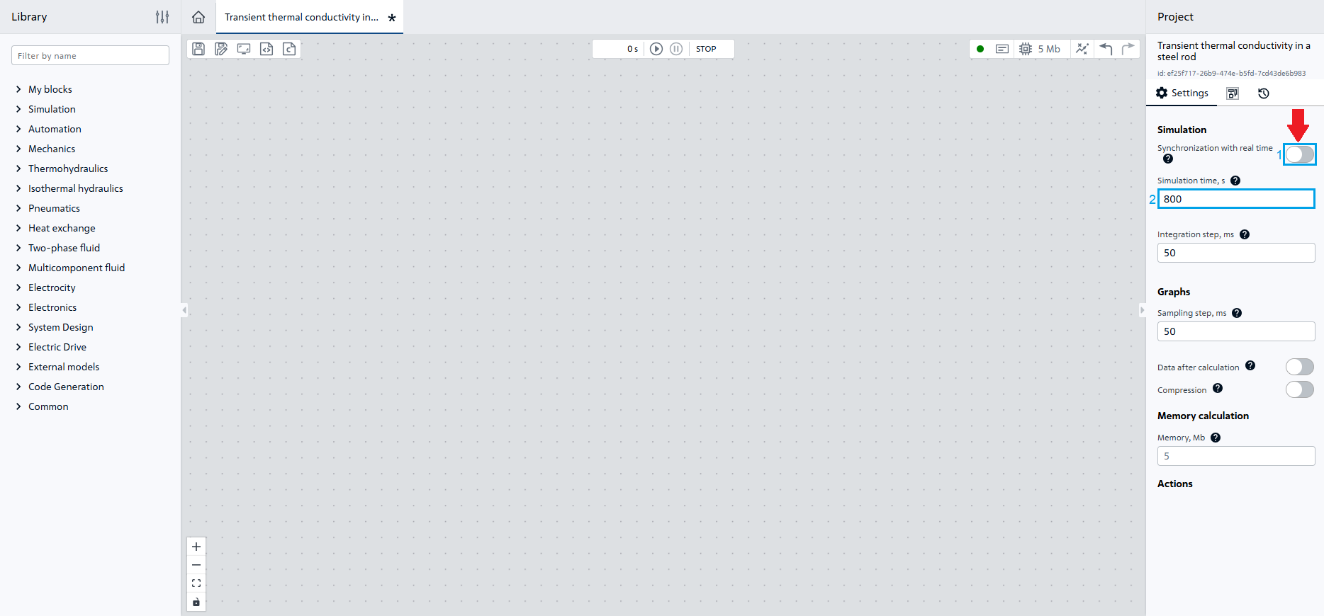
Fig. 2 Project settings configuration#
Let’s begin the basic steps for creating a thermal model.
2. Setting boundary conditions#
The temperature at the left end of the rod is set and equal to 100℃ (source temperature). In order to simulate this boundary condition, use the Temperature source block of the Heat exchange library, place it in the workspace and set the temperature value with the block [Constant of the Automation library by similarly adding it to the workspace and assigning Constant value 100 in its properties.
Let’s connect the blocks as shown in the Fig. 3:
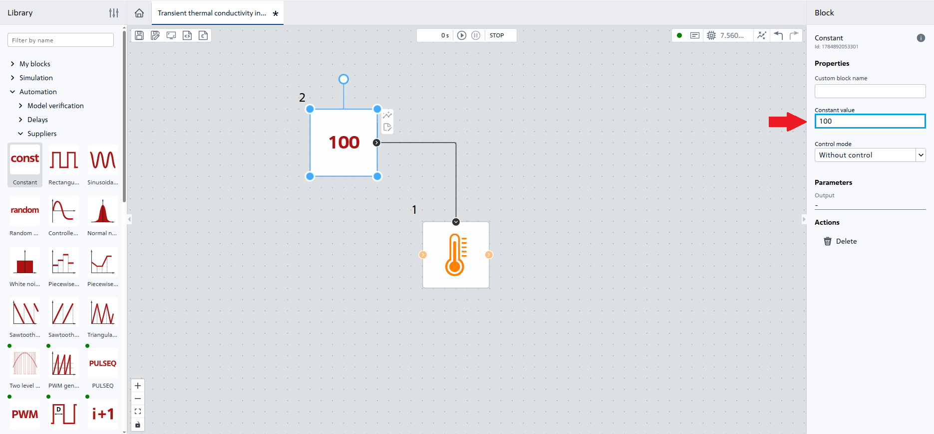
Fig. 3 Setting the temperature using the Constant block#
3. Rod simulation#
In this problem, we want to demonstrate the process of heating the rod. The user can choose the level of detail independently, in the tutorial the rod is divided into 4 parts, Fig. 4:
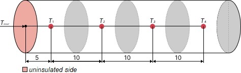
Fig. 4 Rod separation diagram#
In order to simulate rod components, add 4 identical blocks Thermal mass of the Heat exchange library with the following properties (see Fig. 5 below):
Specific heat type-Table of values;Mass- 0.006205 [kg];
Hint
The mass of one segment is equal to 0.006205 [kg] (1/4 part of the total mass of the rod).
Initial temperature- 25℃;Specific thermal capacity curve- set the values from the second columnSpecific heat capacity curveof the tableSpecific thermal capacity;Temperature curve- set the values from the first columnTemperatureof theSpecific thermal capacitytable.
Important
In REPEAT VISION, decimal numbers are specified through a period.
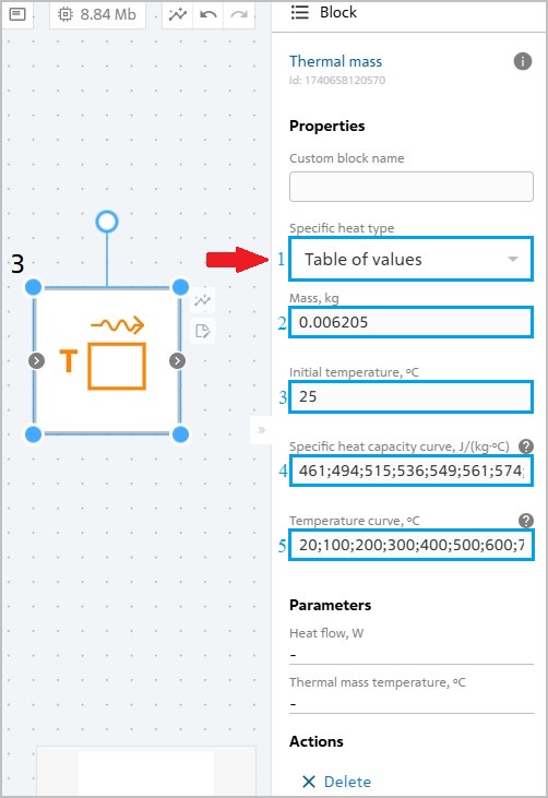
Fig. 5 Setting Thermal mass block properties#
Select block Thermal mass by LMB, then pressing the keyboard shortcuts Ctrl+C once and Ctrl+V three times, create 3 more copies of this block with completely identical properties, Fig. 6:</a
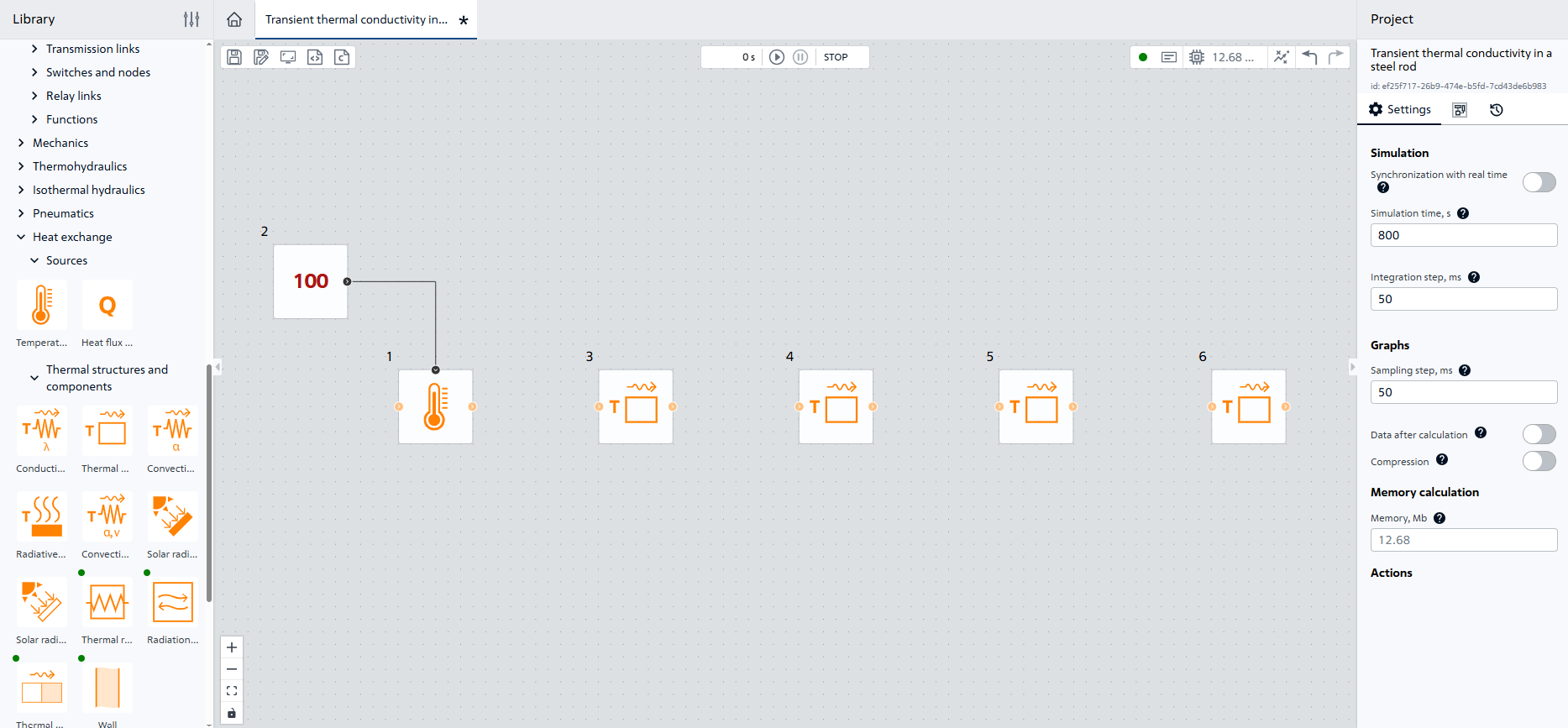
Fig. 6 Location of four blocks Thermal mass#
Each thermal mass is one part of the rod, the heat between them is distributed through thermal conductivity.
In order to simulate heat transfer between parts, add four blocks Conductive heat transfer with the following properties (see Fig. 7 below):
1.Surface area - 0.00007854 [m\(^2\)];
2. Wall thickness - 0.01 [m];
3. Conductivity type - Table of values;
4. Thermal conductivity curve - set the values from the second column Thermal conductivity of the Thermal conductivity table;
5. Temperature curve - set the values from the first column Temperature of the Thermal conductivity table.
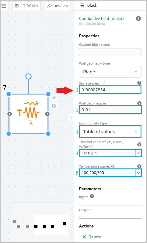
Fig. 7 Properties of Conductive heat transfer blocks#
After setting the above properties for the first Conductive heat transfer block, we will make 3 more copies, similar to creating copies of the block Thermal mass. After creating blocks №7, 8, 9 and 10 (Conductive heat transfer blocks), one shall change the Wall thickness property of block №7 to 0.005 [m], because in this case the wall thickness is half the length of the segment according to the schematic diagram, Fig. 8 и Fig. 9:
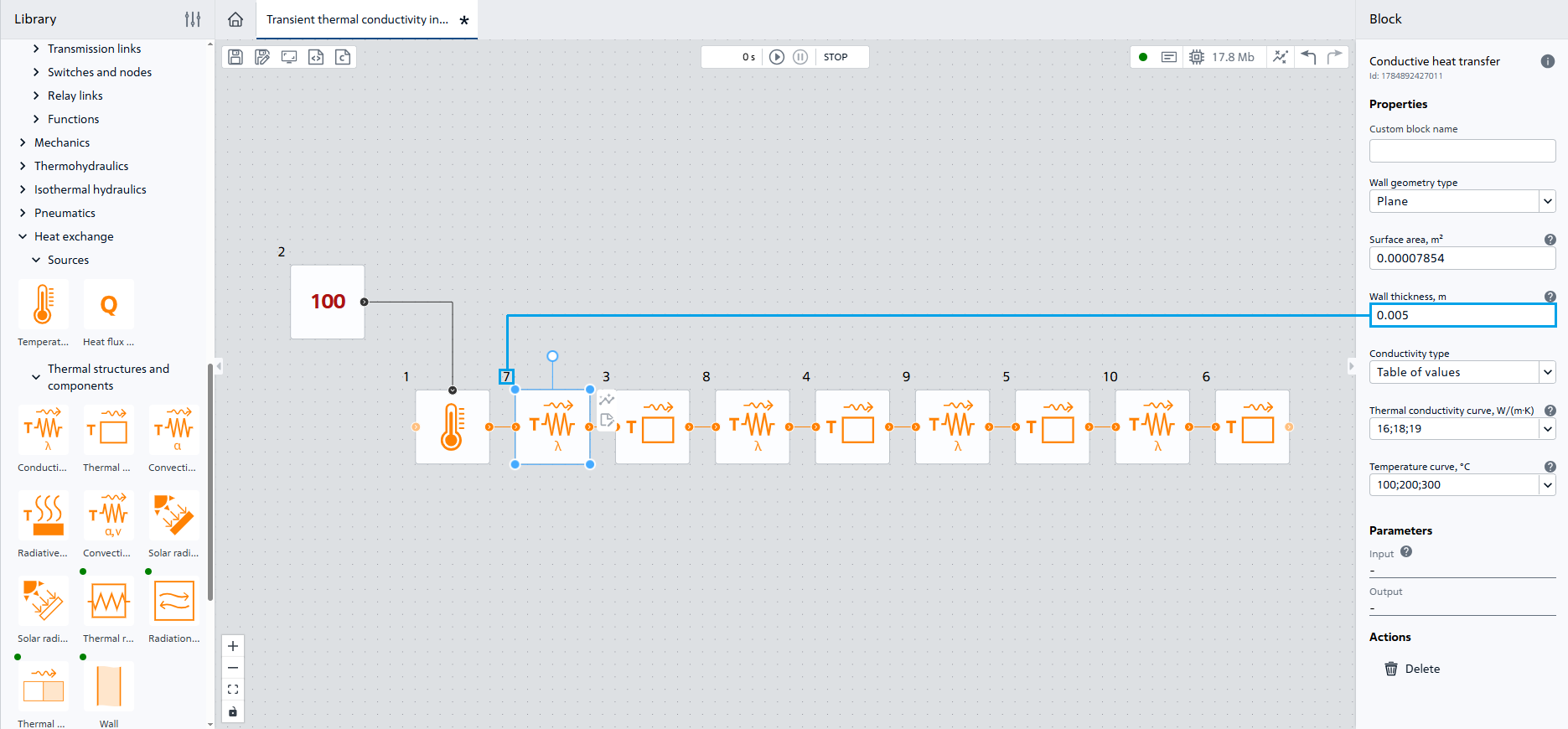
Fig. 8 Connecting blocks and changing the value of the property of block №7 Conductive heat transfer#
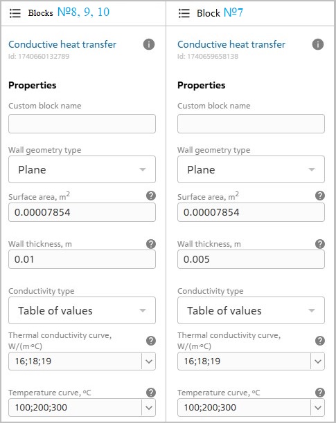
Fig. 9 Differences in Conductive heat transfer block properties#
4. Output of calculation results#
Add the rod segments temperature change charts using the visualization panel (see Fig. 10 below):
Click on the
Visualizationbutton located on the bottom panel on the left;Double-click on the
Addbutton located in the lower right corner to add two charts;In the first chart window, click on the
Block parameters, axis Ypanel and select all four Thermal mass blocks there;In the second chart window, click on the
Block parameters, axis Ypanel similar to item 3 and select all four Conductive heat transfer blocks there.
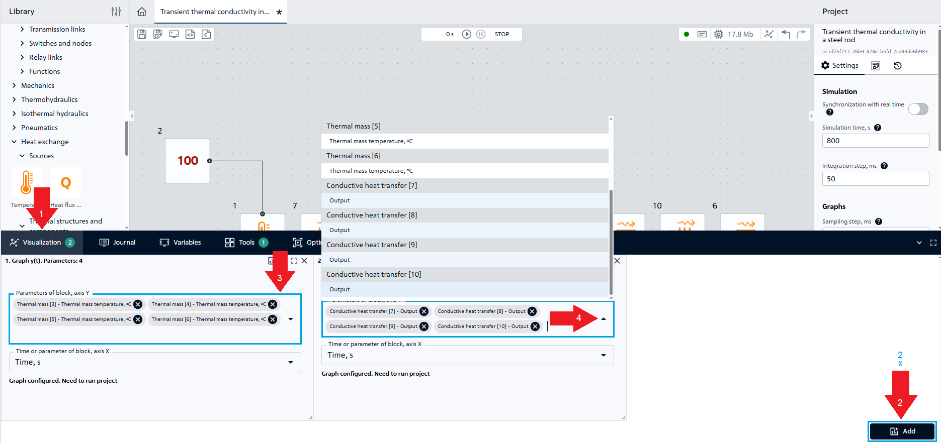
Fig. 10 Adding charts#
Save the project.
The thermal model is ready for calculation.
5. Calculation start#
Start calculation using the “Start simulation”  button
The calculation should be successfully completed with the following message:
Modeling stopped on the solver side due to modeling time limit exceeded.
6. Analysis of calculation results#
As a result of simulation, we obtain charts of changes in segment temperatures, as well as heat fluxes for thermal conductivity blocks, Fig. 11:
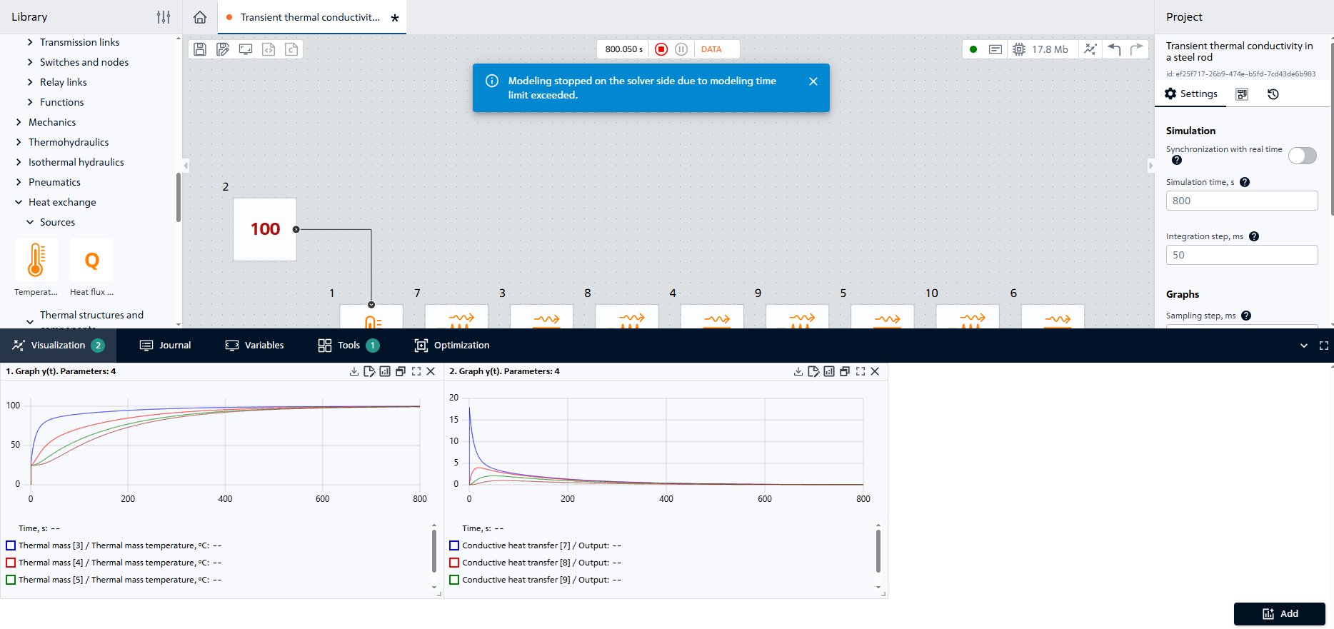
Fig. 12 Charts#
The temperature change of the first segment is much faster than the others, since this segment is located closer to the temperature source.
At the initial time, the heat fluxes between 1 and 2, 2 and 3, 3 and 4 are zero due to the absence of temperature difference. In turn, there is heat flow between the source and segment 1 at the initial moment, since this segment is directly connected to the source and the temperature difference is available.
7. Conclusions#
In this tutorial, you learned how to simulate transient heat transfer processes using the Heat exchange library blocks.
You have learned how to:
Obtain charts of element temperature changes;
Detail the item into segments and build thermal links between them;
Set non-constant material properties (specific thermal capacity, thermal conductivity).