

Plotting of pump pressure characteristic#
This tutorial describes simple steps for modeling a system for pumping liquid at atmospheric pressure from the first tank with hot water of 52℃, to the second tank with a temperature of 20℃.
Water is supplied to the tank using pumps having parameters at the operating point:
flow rate – 600 [m\(^3\)/hour];
head – 60 [m].
The diameter corresponds to 420 [mm]. Flow and pressure characteristics are shown in Fig. 1:
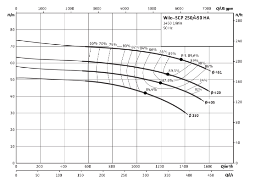
Fig. 1 Pump pressure characteristic#
We consider a problem in which it is required to plot the pressure characteristic of a pump, by creating resistance in the mains by a hydraulic orifice of variable diameter.
1. Project creation#
To begin with, create a new project and name it, e.g. Build pump pressure characteristic.
Let us proceed with the basic steps to create the circuit by opening the library Thermohydraulics
2. Adding tanks#
Move to the workspace blocks №1-2. For this purpose, move block Reservoir (TL) to the workspace and give it the following values property:
Value |
|
|---|---|
1 Gauge pressure |
0 [Pa] |
2 Temperature |
52°C |
0.1764 [m\(^2\)] |
Note
Through cross-section of the ports corresponds to the area of the pipeline.
Important
At REPEAT VISION decimal numbers are set through a period.
We will need two of these blocks, for this we will use one of the methods ..
To do this, drag block №2 on to the workspace.
This requires:
Select
block №1with the left mouse button;Press the CTRL+C and CTRL+V buttons.
Note
The second method is preferable, since all the property values of blocks №1 and №2, except for Temperature, °C, are the same.
Change the value of property of Temperature, °C of block №2 relative to the values of properties of block №1.
Value |
|
|---|---|
1 Temperature |
20°C |
Values of properties of blocks №1-2, Fig. 2:
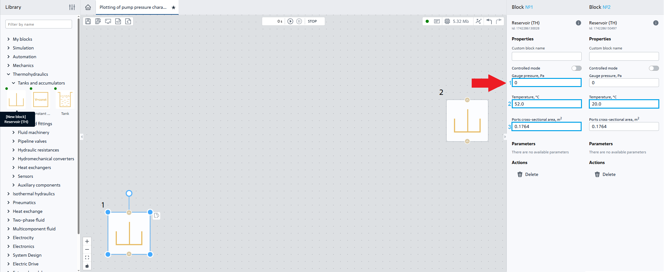
Fig. 2 Properties of blocks №1-2#
3. Adding an orifice#
Let’s move block №3 Orifice (TL) to the working area and specify the following properties for it:
Property |
Value |
|---|---|
1 Port area |
0.1764 [m\(^2\)] |
2 Orifice area vector |
0.0025; 0.005; 0.01; 0.015; 0.02; 0.03; 0.04; 0.05; 0.1; 0.17 [м\(^2\)] |
Note
The other properties of block №3 should be remained unchanged
Values of properties of block №3, Fig. 3:
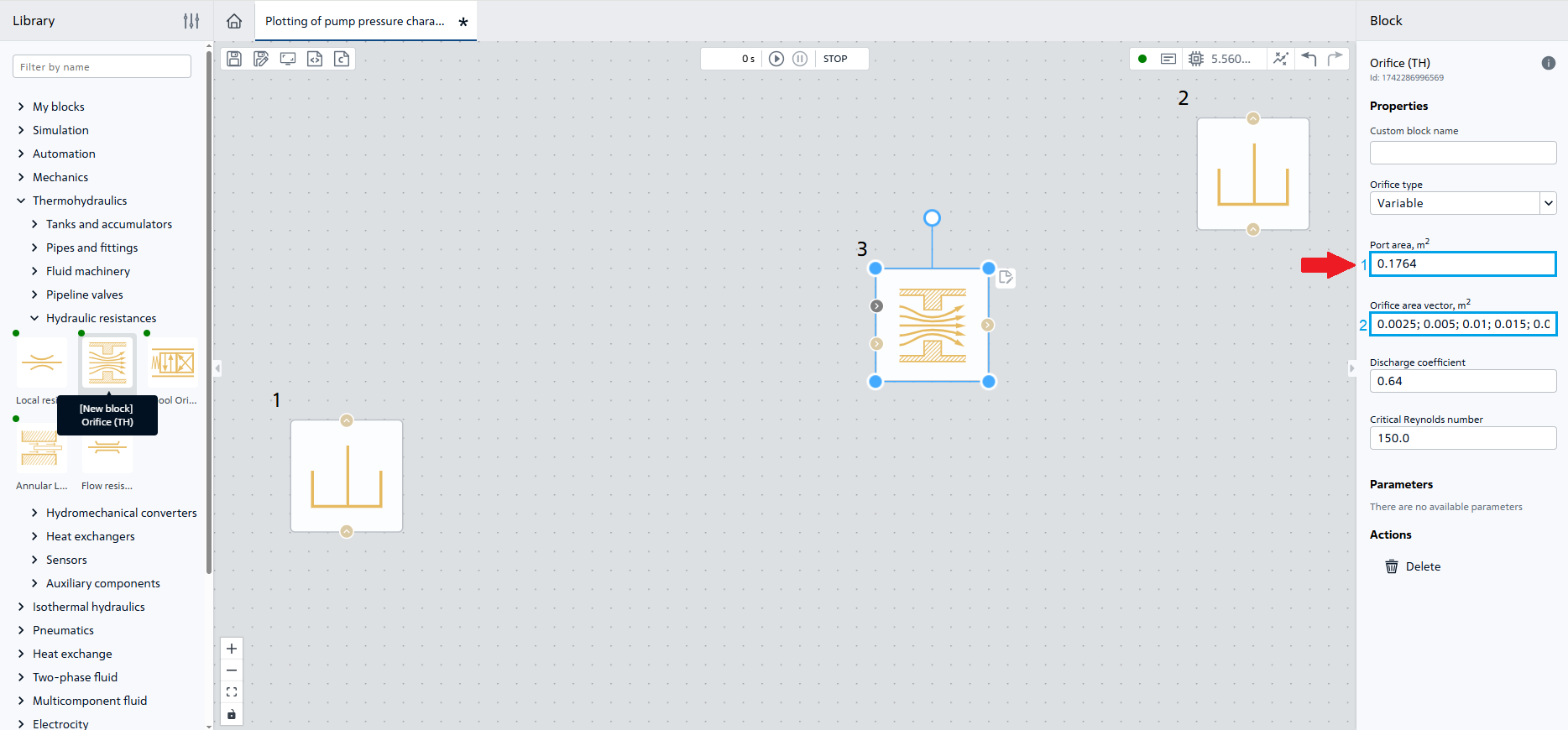
Fig. 3 Properties of block №3#
4. Adding a pump#
Move to the workspace block №4 Tabulated pump (TL) and give it the following properties:
Property |
Value |
|---|---|
1 Port area |
0.1764 [m\(^2\)] |
2 Reference head vector |
65; 63; 62; 60; 59; 56; 50; 0 [m] |
3 Capacity vector |
0; 3333; 6666; 10000; 13333; 16666; 20000; 36666 [lpm] |
Note
The last property of block №4 should be remained unchanged
Property values of block №4, Fig. 4:
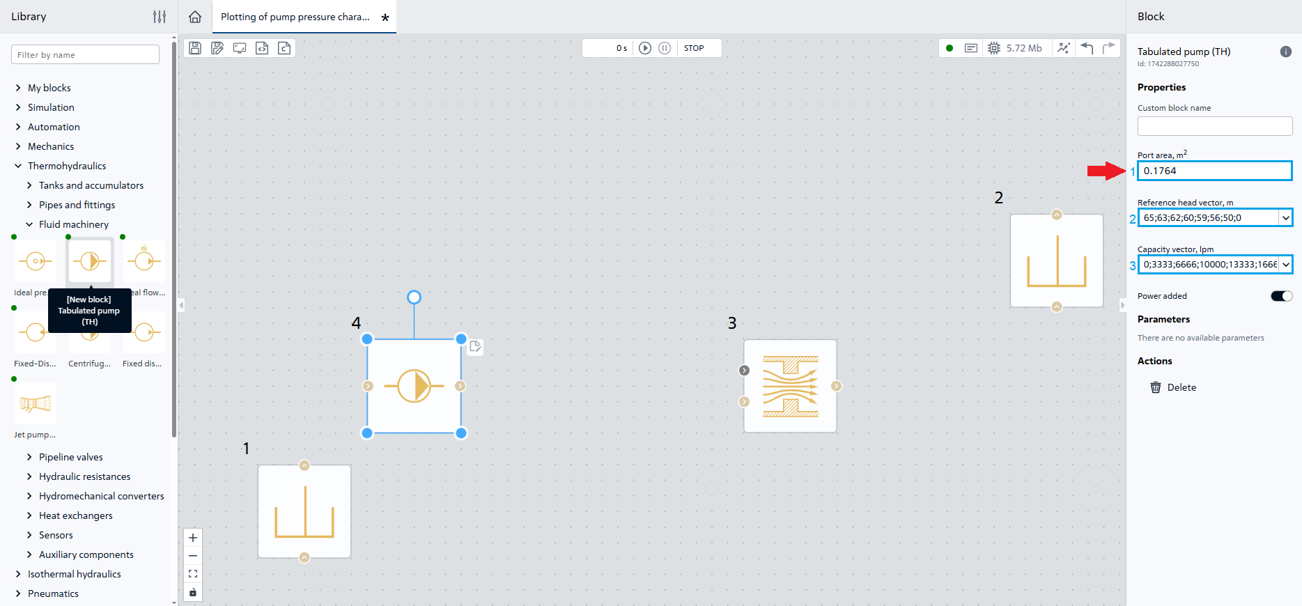
Fig. 4 Properties of block №4#
5. Adding a pipeline section#
Move to the workspace block №5 Pipe (TL) and give it the following properties:
Property |
Value |
|---|---|
1 Pipe length |
20 [m] |
2 Pipe diameter |
0.42 [m] |
Note
The other properties of block №5 should be remained unchanged
Values of properties of block №5, Fig. 5:
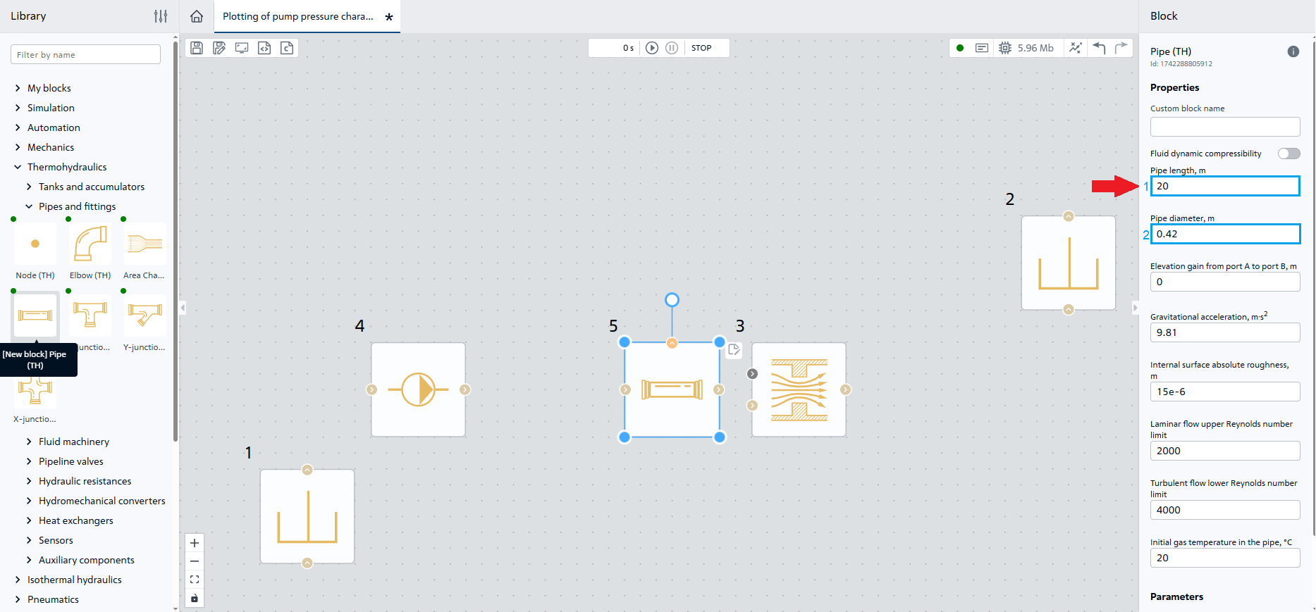
Fig. 5 Properties of block №5#
6. Adding nodes#
Move to the workspace blocks №6–7. To do this, move to the workspace block Node (TL) and give it the following property value:
Property |
Value |
|---|---|
1 Number of input ports |
1 |
Note
The last property of block №6 should be remained unchanged
We will need two of these blocks, we will use one of the methods to do this.
Hint
The second way is also preferred
Values of properties of blocks №6-7, Fig. 6:
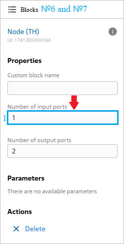
Fig. 6 Properties of blocks №6-7#
7. Adding sensors#
Move to the workspace
block №8Flow Rate Sensor (TL)and select in its propertyRelated block-Pipeline section (TL), Fig. 7:
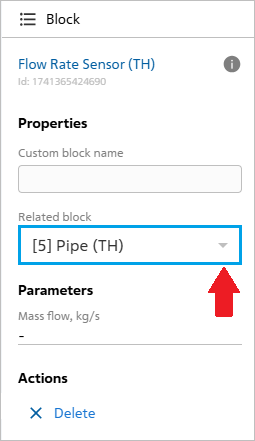
Fig. 7 Property of block №8#
Move to the workspace
blocks №9–10Pressure and temperature sensor (TL):
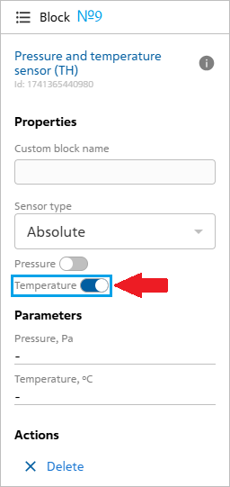
Fig. 8 Property of block №9#
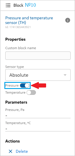
Fig. 9 Property of block №10#
Place and connect the blocks according to the Fig. 10:
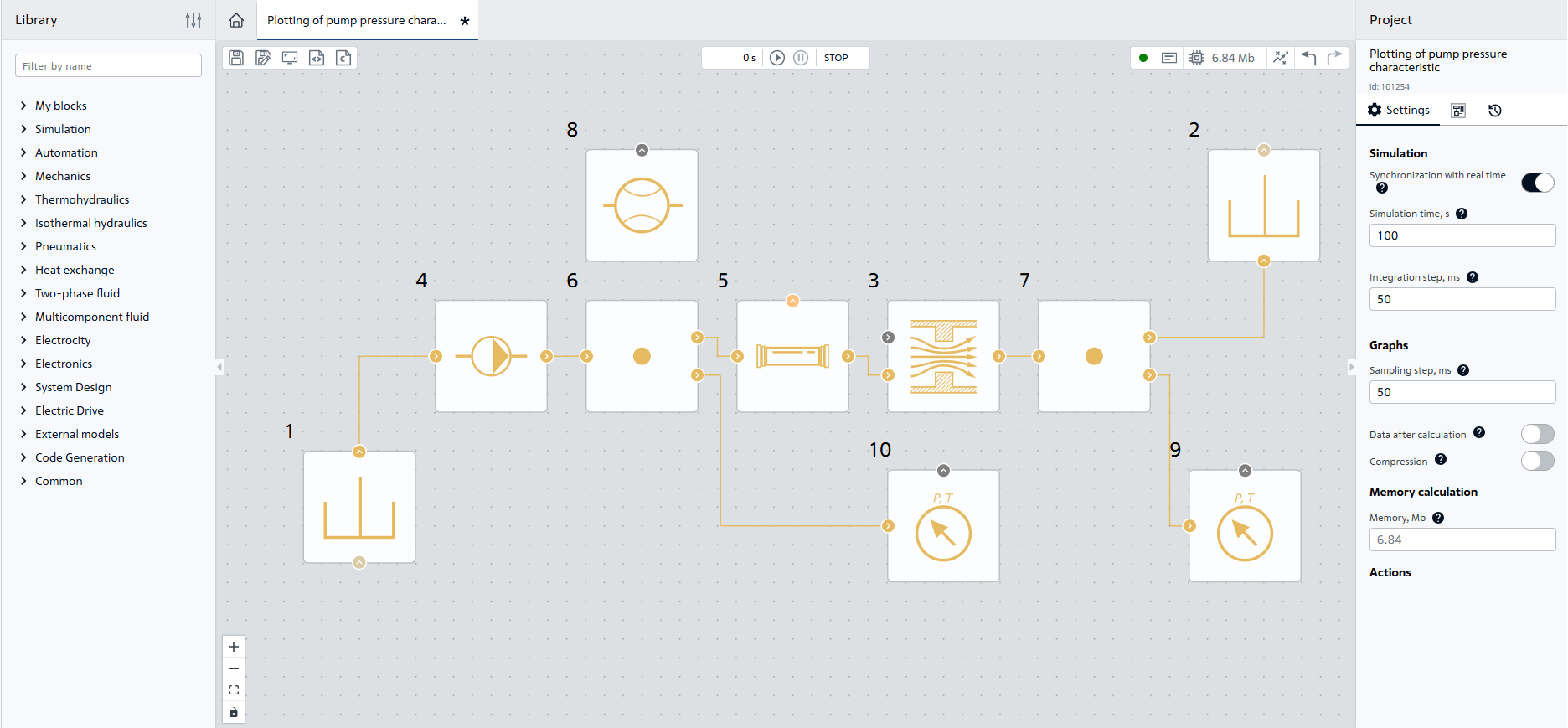
Fig. 10 Placement and connection of TL blocks#
8. Adding a control signal#
Move to the workspace block №11 Piecewise-linear function connect it to the circuit and specify the following properties:
Property |
Value |
|---|---|
1 Vector of time arguments |
0; 30; 50 [s] |
2 Vector of function values |
0; 0.5; 1 |
3 Periodicity |
|
Place and connect the block according to the Fig. 11:
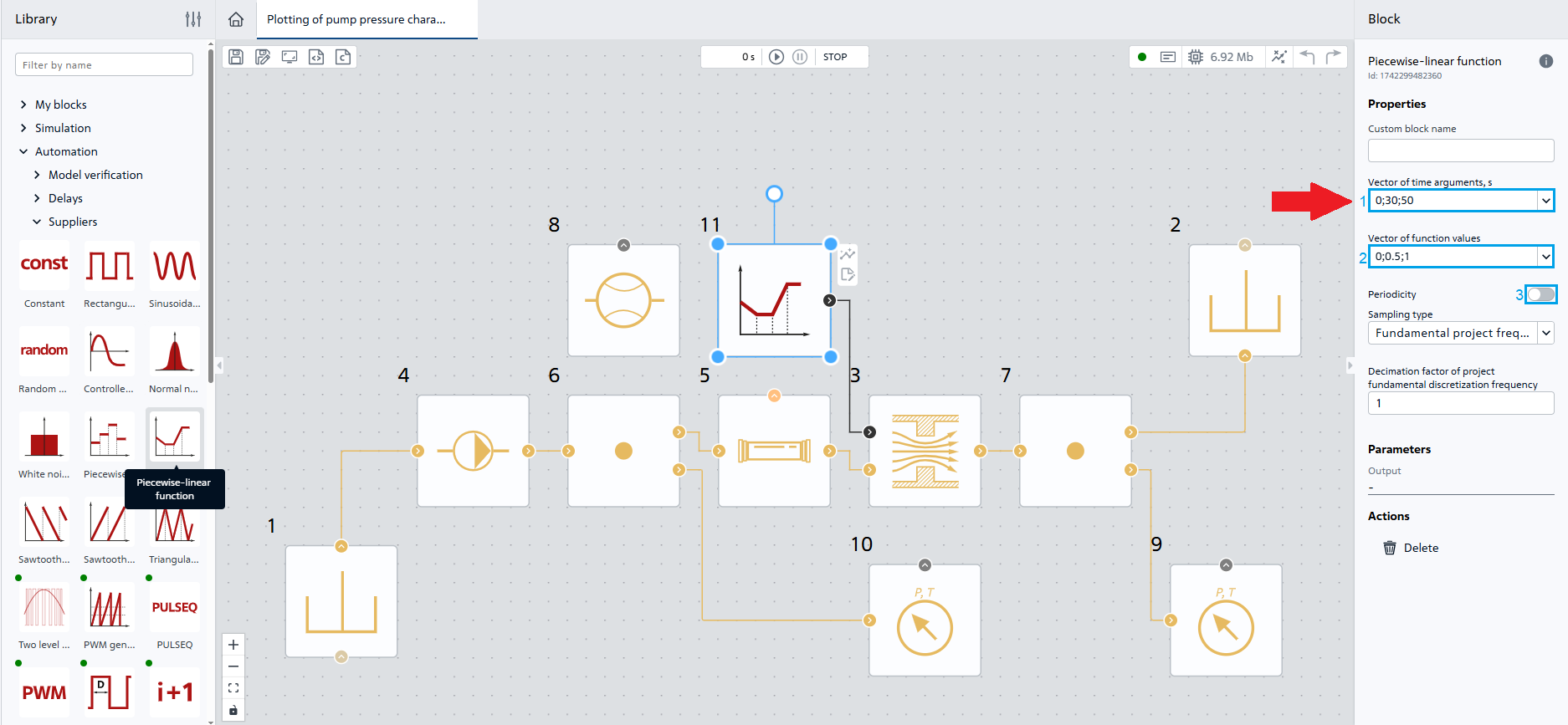
Fig. 11 Connection of block №11 and its properties#
9. Add graphs for visualization#
Go to the Visualization tab (see Fig. 12 below);
Add two graphs by double-clicking on the Add button in the lower right corner;
In the first graph window, click on
Block parameter, Y axis- selectPressure, Pa;Then in the first graph window, click
Time or block parameter, X axis- selectMass flow rate, kg/s;Then in the second graph window, click
Block parameter, Y axis- selectTemperature, °C.
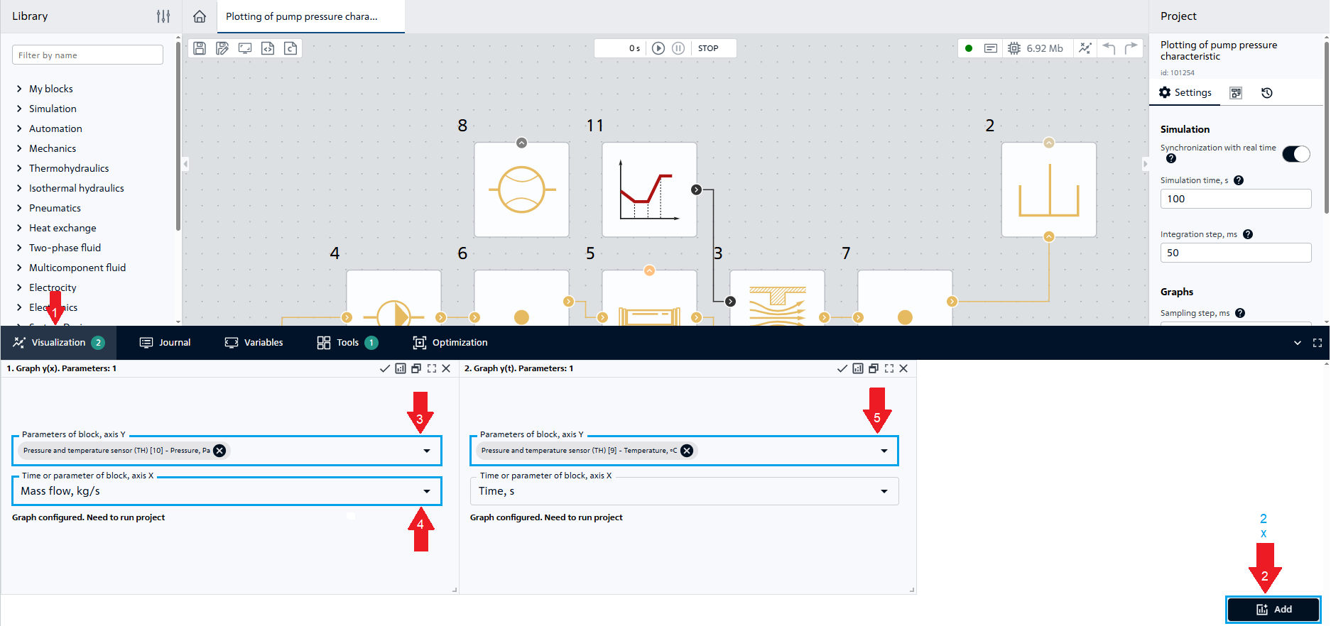
Fig. 12 Visualization#
Run the calculation by the “Run Simulation” button 
The calculation shall be successfully completed with the following message:
Modeling stopped on the solver side due to modeling time limit exceeded.
10. Analysis of calculation results#
The previously created graph 1 should now display the pump pressure characteristic, Fig. 13:
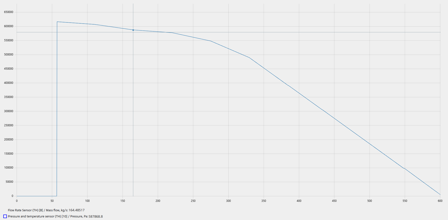
Fig. 13 Pump pressure characteristic - pump operating point#
Block Orifice (TL) serves as a resistance for the pump in the mains. Over time it slightly opens from 0 to 1, controlled by the signal of the block Piecewise-linear function.
On graph of pump pressure response it can be seen that a lower flow rate corresponds to a higher pressure generated by the pump. Lower pressure results in higher flow rates. At the pump operating point, at a flow rate of 600 [m\(^3\)/h], with a water temperature of 52˚C, the density is 987.2 [kg/m\(^3\)], and the flow rate is 164.5 [kg/s].
\(G=\frac{Q\cdot \rho}{3600}=\frac{600[м^3/ч]\cdot987.2[кг/м^3]}{3600[с]}=164.5[кг/с]\)
A head of 60 [m] at a water temperature of 52˚C corresponds 581066 [Pa].
\(P= ho \cdot g \cdot h=987.2[kg/m^3]\cdot 9.81[m/s^2]\cdot 60[m]=581066[Pa]\) - Pump operating point
On graph the excess pressure at the point behind the pump is 581420 [Pa], at the pump inlet the pressure is atmospheric, the difference is 581420 [Pa].
\(\frac{|P-P_{мод}|}{P}\cdot 100\)%=\(\frac{|581066-581420|}{561066}\cdot 100\)%=0.06%
On graph (see Fig. 14 below) of temperature we can see a smooth temperature increase in the detail, when the block hydraulic opening is opened by 50%, the temperature is 47.72˚C, corresponding to a flow rate of 431 [kg/s]. When fully opened in 70 [s], the temperature goes to 52˚С.
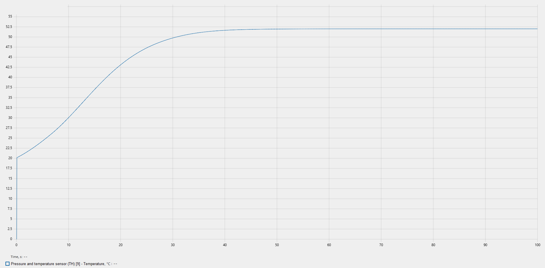
Fig. 14 Water temperatures from time#
11. Summary#
During this tutorial you have gained basic knowledge for modeling in the software REPEAT VISION by blocks Thermohydraulics, in particular:
Orifice (TL)with variable section area.
Herein the pressure characteristic of the pump was plotted, the operating point was compared with the graph, the measurement error is about zero, we can conclude that the pump unit is operating correctly.