

Orifice (TL)#
Block appearance in REPEAT VISION#
The Orifice (TL) block models flow through a local restriction with a constant orifice area. The orifice area is parameterized either linearly or using a lookup table.
The block conserves mass such that (1):
This mass balance implies that velocity increases as the area decreases and decreases when the flow discharges into a larger area. According to Bernoulli’s principle, this velocity change results in a region of lower pressure in the orifice and higher pressure in the expansion zone. The resulting pressure increase, referred to as pressure recovery, depends on the pressure recovery loss coefficient and the ratio of the orifice area to the port area.
Mass Flow Calculation
The block calculates mass flow as (2):
where:
\(C_d\) – discharge coefficient;
\(A_{orifice}\) – orifice area, [m\(^2\)];
\(A_{port}\) — cross-sectional area of ports A and B, [m\(^2\)];
\(\barρ\) – average fluid density, [kg/m\(^3\)].
Pressure Loss
Pressure loss describes the pressure drop in the valve due to the area reduction. The pressure loss, PRloss, is calculated as (3):
Critical Pressure
The critical pressure drop, \(Δp_{crit}\), is the pressure drop associated with the critical Reynolds number, Re\(_{crit}\), which marks the transition between laminar and turbulent flow in the fluid (4):
Law of conservation of energy (5):
1. Procedure for using variable orifice area in the block#
The Orifice (TL) block allows the use of variable orifice area values.
The change in area is controlled by an automation signal (in this scheme from block №14) within the range [0 to 1]. A value of 0 corresponds to the first value in the orifice area vector, while a value of 1 corresponds to the last. Intermediate values are interpolated according to a piecewise function defined by the vector .
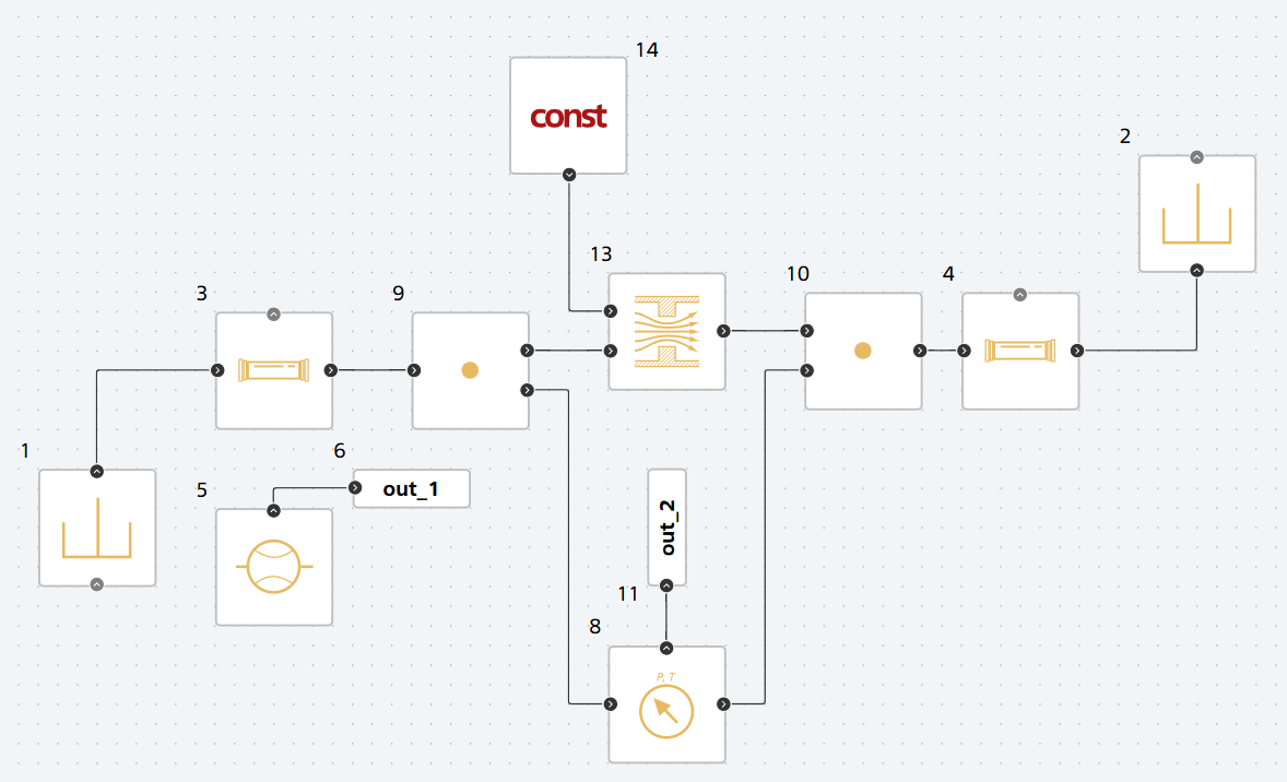
Example of a hydraulic orifice with adjustable area:#
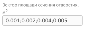
Example list of orifice area values#
2. Properties#
Property |
Default Value |
Description |
Units of measurement |
|---|---|---|---|
Orifice type: |
Variable |
- |
- |
Port area |
0.001 |
- |
m\(^2\) |
Orifice area, available when selecting |
1.0E-4 |
- |
m\(^2\) |
Orifice area vector, available when selecting |
{1.0E-9; 2.0352E-7; 4.0736E-5; 1.1438E-4; 3.4356E-4;} |
- |
- |
Discharge coefficient |
0.64 |
- |
- |
Critical Reynolds number |
150.0 |
- |
- |
3. Inputs and outputs#
Parameters |
Input/Output |
Description |
Units of measurement |
Port type |
|---|---|---|---|---|
Spool displacement |
Input |
Available, when |
m |
Automation |
Input |
Input |
- |
- |
Thermohydraulics |
Output |
Output |
- |
- |
Thermohydraulics |
In order to see the connection capabilities of the block, you need to go to page Description of block ports
See also
An example of using this block can be found in the tutorial of the library Thermohydraulics: