

T-junction (IH)#
Block appearance in REPEAT VISION#
TheT-junction (IH) block simulates the junction of three branches of the hydraulic network at an angle of 90\(^о\). To calculate the loss coefficients at the junction of flows, one can choose one of three correlation options in accordance with the values of Loss coefficient model property:
According to Crane;
According to Rennel;
Custom.
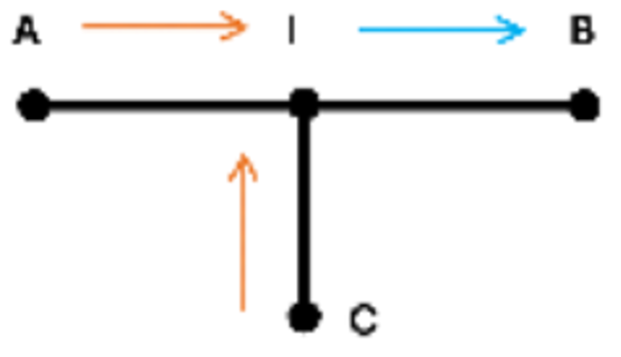
Fig. 1 Flow converging to vertex B#
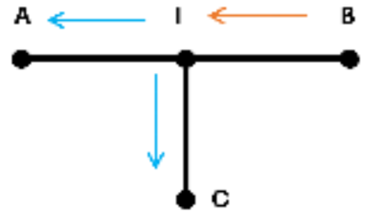
Fig. 2 Flow diverging from vertex B#
Hint
The AIB branch is the main one, the CI branch is the side one.
1. Crane’s Loss Calculation#
The loss coefficients for converging and diverging flows are equal and are defined for the main and side branches as follows (1), (2) :
where the dimensionless coefficients \(f_T\) for the side and main branch depend on the corresponding diameters and are calculated as per the table by interpolation method:
Nominal size, mm |
5 |
10 |
15 |
20 |
25 |
32 |
40 |
50 |
72.5 |
100 |
125 |
150 |
225 |
350 |
609.5 |
|---|---|---|---|---|---|---|---|---|---|---|---|---|---|---|---|
Friction coefficient, \(f_T\) |
0.035 |
0.029 |
0.027 |
0.025 |
0.023 |
0.022 |
0.021 |
0.019 |
0.018 |
0.017 |
0.016 |
0.015 |
0.014 |
0.013 |
0.012 |
2. Rennel’s Loss Calculation#
The loss coefficients for converging and diverging flows on the main and side branch are defined as (3), (4), (6), (9), (11), (12) :
where \(K_*\) is calculated as (5)
where \(С_M\) and \(C_{xC}\) coefficients are calculated as (7), (8) :
where coefficient \(C_{yC}\) is calculated as (10) :
Hint
All the above coefficients are dimensionless.
User Loss Factors:
With this setting, the user directly sets dimensionless loss coefficients for converging and diverging flows on the main and side branches:
\(K_{main,conv}\) – divergent flow on the main branch;
\(K_{main,div}\) – converging flow on the main branch;
\(K_{side,conv}\) – divergent flow on the side branch;
\(K_{side,div}\) – converging flow on the side branch.
Mass conservation equation(13) :
Pressure drop calculation (14), (15), (16) :
where:
\(A_{main}\) – main branch cross-sectional area, [m\(^2\)];
\(A_{side}\) – side branch cross-sectional area, [m\(^2\)];
\(K_A, K_B, K_C\) – dimensionless loss coefficients on branches AI, BI, CI respectively;
\(I_A, I_B, I_C\) – liquid inertia on branches AI, BI, CI respectively;
\(m_A, m_B, m_C\) – mass flow rate of liquid through ports A, B, C, respectively, [kg/s].
\(m_{thresh}\) – threshold flow rate, below which the flow is considered stagnant and cannot be defined as converging or diverging. Calculated using the following formula (17) :
where:
\(A_{min}\) – minimum area of the side and main branches, [m\(^2\)];
\( ho\) – liquid density, [kg/m\(^3\)];
\( u\) – liquid kinematic viscosity, [mm\(^2\)/s].
Calculation of inertia (18), (19), (20) :
3. Properties#
Property |
Default Value |
Description |
Units of measurement |
|---|---|---|---|
Loss coefficient model: |
Crane |
- |
- |
Main branch area |
0.01 |
- |
m\(^2\) |
Side branch area |
0.01 |
- |
m\(^2\) |
Junction radius, available when selecting |
0.5 |
- |
m |
Critical Reynolds number |
150.0 |
- |
- |
Minimum flow ratio, available when selecting |
0.2 |
- |
- |
Loss coefficient for main branch (convergence flow), available when selecting |
1.12 |
- |
- |
Loss coefficient for main branch (divergence flow), available when selecting |
1.12 |
- |
- |
Loss coefficient for side branch (convergence flow), available when selecting |
1.12 |
- |
- |
Loss coefficient for side branch (divergence flow), available when selecting |
1.12 |
- |
- |
4. Inputs and outputs#
Parameters |
Input/Output |
Description |
Units of measurement |
Port type |
|---|---|---|---|---|
Port A |
Input |
- |
- |
Isothermal Hydraulics |
Port B |
Input |
- |
- |
Isothermal Hydraulics |
Port C |
Input |
- |
- |
Isothermal Hydraulics |
In order to see the connection capabilities of the block, you need to go to page Description of block ports