Local resistance (TL)#

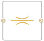
block — Block appearance in REPEAT VISION#

Local resistance (TL) unit simulates pressure loss due to user-defined pipe resistances in the thermal hydraulic network.

Hint

You can specify different loss factors for forward and reverse flows through a pipe segment.

The loss factor is parameterized either by a constant relationship based on pipe pressure or by user-provided tabular data for loss factors based on Reynolds number.

1.Loss coefficient

a) Constant loss coefficient

Segments with loss factors that remain constant over a range of flow rates are calculated as (1):

(1)#\[ k_{loss}\:=\:k_{loss,BA}+\frac{k_{loss,AB}\:-\:k_{loss,BA}}{2}\:\cdot\:\tanh{(\frac{3\:\:\Delta p}{\Delta p_{crit}}+1)} \]

where:

$k_{loss,AB}$ and $k_{loss,BA}$ — parameters of forward flow loss factor (from A to B) and return flow loss factor (from B to A), respectively.

$Δp$ – pressure difference $p_A$ – $p_B$, [Pa].

Critical pressure differential, $Δp_{crit}$, is the pressure differential associated with the critical Reynolds number, $Re_{crit}$, which is the transition point of the flow condition between laminar and turbulent flow (2):

(2)#\[ \Delta p_{crit}\:=\:\frac{\bar{\rho}}{2} k_{loss,crit}\:\:(\frac{\nu\:\cdot\:Re_{crit}}{D_{h}})^2 \]

where:

$k_{loss,crit}$ — is the loss coefficient associated with critical pressure, which is based on the average of the forward and reverse loss factors;

$v$ - liquid kinematic viscosity, [m$^2$/s];

$ρ$ – average liquid density, [kg/m$^3$];

$Dh$ – hydraulic diameter of the segment, [m], which is the equivalent diameter of the non-circular pipe $D_{h}\:=\:\sqrt{\frac{4\:A_{flow}}{\pi}}$;

$A_{flow}$ — flow area, [m$^2$].

b) Loss coefficient table

The loss factor may alternatively be interpolated based on user-provided Reynolds numbers and loss factor data. A vector of Reynolds numbers can have both positive and negative values, indicating forward and backward flow, respectively (3):

(3)#\[ k_{loss}\:=\:f(Re) \]

2. Mass flow rate calculation

Law of conservation of mass (4):

(4)#\[ \dot m_{A}+\dot m_{B}\:=\:0 \]

The mass flow rate through the resistance is calculated as (5):

(5)#\[ \dot m\:=\:A_{flow}\:\:\sqrt{\frac{2\:\bar{\rho}}{k_{loss}}}\:\:\frac{\Delta p}{(\Delta p^2 + \Delta p_{crit}^2)^{1/4}} \]

where $k_loss$ is the flow loss factor that is chosen between the forward flow loss factor (A to B) and the reverse flow loss factor (B to A) depending on the flow direction of the unit.

3. Energy balance

Law of conservation of energy (6):

(6)#\[ \phi_{A}+ \phi_{B}\:=\:0 \]

where:

$\phi_А$ - energy flow at the input, [W];

$\phi_В$ - energy flow at the output, [W].

1. Properties#

Property	Default value	Description	Units of measurement
Method of loss calculation: Constant coefficients; Variable coefficients; Tabulated data: K$_{loss}$ = f(Re); Tabulated data: dP = f(m’)	Constant coefficients	-	-
Straight flow loss coefficient, available when selecting `Method of loss calculation` - `Constant coefficients`	1.0	-	-
Reverse flow loss coefficient, available when selecting `Method of loss calculation` - `Constant coefficients`	1.0	-	-
Reynolds numbers vector, available when selecting `Method of loss calculation` - `Tabulated data: K$_{loss}$ = f(Re)`	-500.0;-200.0;-100.0;-50.0;-40.0;-30.0; -20.0;-10.0;10.0;20.0;30.0;40.0;50.0;100.0; 200.0;500.0;1000.0;2000.0;	-	-
Loss coefficient vector, available when selecting `Method of loss calculation` - `Tabulated data: K$_{loss}$ = f(Re)`	0.65;0.75;0.9;1.15;1.35;1.65; 2.3;3.1;4.0;2.7;1.8;1.46; 1.3;0.9;0.65;0.42;0.3;0.2;	-	-
Pressure drop vector, available when selecting `Method of loss calculation` - `Tabulated data: dP = f(m')`	1272.0;3000.0;4128.0; 6150.0;7718.0;10400.0;	-	Pa
Mass flow vector, available when selecting `Method of loss calculation` - `Tabulated data: dP = f(m')`	0.105;0.175;0.21; 0.2625;0.2975;0.35;	-	kg/s
Flow area	0.2	-	m$^2$
Critical Reynolds number	150.0	The Reynolds number at which the transition from laminar to turbulent flow occurs	-

2. Inputs and outputs#

Parameters	Input/Output	Description	Units of measurement	Port type
Input	Input	-	-	Thermohydraulics
Output	Output	-	-	Thermohydraulics
Loss coefficent (straight flow)	Input	Available when selecting `Method of loss calculation` - `Variable coefficients`	-	Automation
Loss coefficent (reverse flow)	Input	Available when selecting `Method of loss calculation` - `Variable coefficients`	-	Automation

In order to see the connection capabilities of the block, you need to go to page Description of block ports

3. Examples of use#

Examples of using this block can be found in the following sections:

Tutorials;
How-to guides;
Description of Demo.

Tutorials

Library	Tutorial name
`Thermohydraulics`	Study of the effect of hydraulic resistance when mixing flows of different temperatures

How-to guides

Section	Guide name
Energy	Development of a model of the industrial circuit system of oil coolers of NPP with WCWR