Electronic DC Motor with Saturation#

The Electronic DC Motor with Saturation block is a model of an electronic DC motor that takes into account the saturation effect of the magnetic system.

Note

The motor model contains two windings: an armature winding and an excitation winding.

The saturation of the magnetic system is taken into account by applying the parameters of the magnetizing curve obtained experimentally.

The model is described by the following equations:

armature winding voltage (1):

(1)#\[u_{ОЯ}=\omega \cdot Ф \cdot C + i_{ОЯ}\cdot R_{ОЯ}+\frac{di_{ОЯ}}{dt}\cdot L_{ОЯ}\]

where:

\(u_{ОЯ}\) – instantaneous voltage value at armature winding terminals, [V];

\(\omega \) – angular speed of armature rotation, [rad/s];

Ф – magnetic flux, [Wb];

C – construction constant (2):

(2)#\[C=\frac{p \cdot N}{2\cdot \pi \cdot a}\]

\(i_{ОЯ}\) – instantaneous value of armature winding current, [А];

\(R_{ОЯ}\) – active resistance of armature winding, [Ohm];

\(L_{ОЯ}\) – inductance of armature winding, [H].

excitation winding voltage (3):

(3)#\[u_{ОВ}=i_{ОВ}\cdot R_{ОВ}+\frac{di_{ОВ}}{dt}\cdot L_{ОВ}\]

where:

\(u_{ОВ}\) – instantaneous voltage value at excitation winding leads, [V];

\(i_{ОВ}\) – instantaneous value of excitation winding current, [A];

\(R_{ОВ}\) – active resistance of excitation winding, [Ohm];

\(L_{ОВ}\) – excitation winding inductance, [H].

mechanics (4):

(4)#\[\frac{d \omega}{dt}\cdot J_Я=M_{вр}-M_{тр}-M_{сн}\]

where:

\(J_Я\) – moment of inertia of armature, [Н\(\cdot m^2\)];

\(M_{rot}\) – electromagnetic torque on armature shaft, [Н\(\cdot\)m];

\(M_{fr}\) - friction torque, [Н\(\cdot\)m];

Note

Determined by friction in bearings and brush-collector device

\(M_{res}\) – moment of resistance created by load on armature shaft, [Н\(\cdot\)m].

Note

This value is supplied to the block from outside via the automatics port and/or the mechanics port.

In equation (1), the product \(\omega \cdot Ф \cdot C \) is the electromotive force (EMF) of the armature. The magnetic flux used herein is determined from the magnetizing curve parameters.

The magnetizing curve is the relationship between the excitation current and the magnetic flux. An example of a magnetizing curve is shown in Fig.1 :

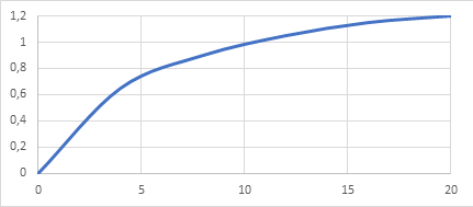
Magnetization_curve_example — Fig. 1 Example of magnetizing curve: horizontal axis - excitation current, [A]; vertical axis - magnetic flux, [Wb]#

The magnetizing curve shall be represented as an array of numerical values (tables with numerical values of each point). Each point in the array represents a pair of values:

excitation current, [A];
magnetic flux, [Wb].

Each point indicates what the magnetic flux is at the specified excitation current. For the magnetizing curve shown in Figure 1, the array of points in steps of 4 [A] is as follows:

\(i_{ОВ}\), [А]	0	4	8	12	16	20
Ф, [Wb]	0	0.65	0.9	1.05	1.15	1.2

Important

One can use any excitation current pitch, including non-constant. However, it should be borne in mind that the more points, the more accurate the simulation of the magnetic system saturation will be.

In the described block, the following requirements are imposed on the array of the magnetizing curve:

the first point should be i\(_{ОВ}\)=0 [А];

Note

The value of the magnetic flux in this case can be any - both positive and negative or equal to zero

there should be no points with the same excitation current value;
each next excitation current value should be greater than the previous one;
the number of excitation current values should be equal to the number of magnetic flux values;
number of points should be at least two.

In the system, the magnetic flux is calculated by interpolating the given values.

For negative excitation current values, the system uses the same array of values, but the excitation current is used with a positive sign and the magnetic flux is generated with a negative sign. Thus, the magnetizing curve is symmetric: the positive branch is similar to the negative one.

The excitation winding inductance used in the equation (3) is determined based on the calculation of the slope of the magnetizing curve using the formula (5):

(5)#\[L_{ОВ}=\frac{dФ}{di_{ОВ}}\cdot n_{кат}\cdot K_{К.П.}=\frac{Ф_1-Ф_2}{\Delta i}\cdot n_{кат}\cdot K_{К.П.}\]

where:

\(Ф_1\) – value of magnetic flux obtained from magnetizing curve at current value of excitation current \(i_{ОВ}\), [Wb];

\(Ф_2\) – magnetic flux value, [Wb], obtained from magnetizing curve at excitation current value equal to (6) :

(6)#\[i=i_{ОВ}+\Delta i\]

\(\Delta i\) – excitation current pitch.

Note

In the considered block, it is assumed that the value of the excitation current pitch \(\Delta i\) is equal to 10% of the current value of the second point of the array. For example, for the array above, the excitation current pitch value would be 0.1\(\cdot\)4=0.4 [А]

\(n_{coil}\) – number of serially connected pole coils.

Note

As a rule, \(n_{coil}\) = 2р - i.e. equal to the number of poles

\(K_{P.D.}\) – pole design factor (7):

(7)#\[K_{К.П.}=w_в\cdot \sigma_в\]

\(w_в\) – number of turns of the pole coil;

\(\sigma_в\) – the dissipation factor of the pole coil

Note

Typically \(\sigma_в\)=1.1 … 1.3

The torques represented by the equation (4) are calculated using the following formulas:

electromagnetic torque on armature shaft (8) :

(8)#\[M_{вр}=i_{ОЯ}\cdot Ф \cdot С\]

friction torque (9) :

(9)#\[M_{тр}=\omega \cdot K_{тр}\]

where \(K_{fr}\) – friction factor.

1. Properties#

Property	Default Value	Description	Units of measurement
Active resistance of the armature winding	2.0	–	Ohm
Armature winding inductance	1e-3	–	H
Active resistance of field winding	5.0	–	Ohm
Motor constant	220.0	\(\frac{p\cdot N}{2\cdot \pi \cdot a}\)	–
Engine friction coefficient	1e-2	–	\((N\cdot m \cdot s)/rad\)
Moment of inertia of the rotor	0.5	-	kg\(\cdot\) m\(^2\)
Initial Conditions Array [Armature winding current, Field winding current, Rotor angular frequency]	0.0; 0.0; 0.0	–	[А; А; rad/s]
Magnetization curve points - Field current	0.0; 4.0; 8.0; 12.0; 16.0; 20.0	Positive values starting from 0	А
Magnetization curve points - Magnetic flux	0.0; 0.65; 0.9; 1.05; 1.15; 1.2	Number of values should be equal to the number of current values	Wb
Number of series-connected main pole coils	2.0	–	units
Dissipation factor of pole windings	10.0	\(w_в \cdot \sigma_в\)	–

2. Inputs and outputs#

Parameters	Input/Output	Description	Units of measurement	Port type
External force torque	Input	Value of shaft torque due to load	N\(\cdot\) m	Automation
+ОЯ	Input	Positive terminal of armature winding	-	Electronics
+ОВ	Input	Excitation winding positive lead	-	Electronics
Angular frequency	Output	Gets connected to angular velocity ports of blocks from the library Mechanics/Rotational motion	rad/s	Rotational motion
-ОЯ	Output	Negative terminal of armature winding	-	Electronics
-ОВ	Output	Negative field lead	-	Electronics

In order to see the connection capabilities of the block, you need to go to page Description of block ports