ODE

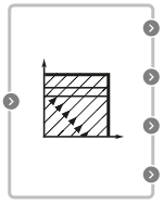
Block appearance in REPEAT VISION

 ODE Block is designed for the numerical solution of systems of ordinary differential equations (ODE) expressed in the Cauchy problem (solved for the highest derivative): \(y" = f(t, y, y')\). The block provides a toolkit for modeling dynamic systems.

Key characteristics and functions of the ODE Block:

• Variable Integration Step Support: To control solution accuracy, algorithms with adaptive step size selection are implemented. Integrators (e.g., Dormand-Prince853, LSODA) automatically adjust the integration step to meet user-specified tolerances (relative and absolute). This is optimal in terms of both speed and accuracy.

• Choice of Integration Scheme: The block offers a set of multi-step and single-step methods (e.g., Runge-Kutta methods of different orders, Adams, LSODA), adapted for solving both non-stiff and stiff problems.

• Event Handling (Discrete Events): An important feature is the ability to process discrete events defined by a condition g(t, y) = 0. The block detects the moment an event occurs, pauses the calculation, allows modification of the state vector, and then resumes the calculation. This is critical for simulating systems with discontinuities (e.g., valve actuation, body collisions) or for stopping integration upon reaching a target state.

• Flexible Event Configuration: The ability to choose the root-finding method for pinpointing the exact moment of an event to improve calculation accuracy and stability.

• Computation Control: A limit on the number of ODE right-hand side function evaluations is set to prevent infinite loops.

• Support for Condition Writing and “Math” Module Import: The block supports conditional operators (if-else) and provides a full set of mathematical functions from the Math module (e.g., Math.sin, Math.exp) for describing the right-hand sides of equations and event conditions.

Operating Principle:

1. The user describes the ODE system by implementing the function \(f(t, y)\).

2. The integrator type is selected and its parameters are configured (tolerances, maximum/minimum step size).

3. The integration process is started.

Important

Although the block’s internal solver uses an adaptive step to guarantee accuracy internally, the entire project executes in a discrete mode. When the overall model calculation step is increased, the ODE solver may require more internal iterations, which necessitates increasing the “Maximum number of function calls” parameter.

 The interface for writing the ODE system generally consists of 6 sections:

• Initialization;

• Main block;

• Additional blocks;

• Integration parameters;

• Extended Event;

• Simple Event.

 In the Initialization section, parameters used in the ODE system calculation are specified, and the initial conditions for the ODE are set: \(y[0] = x_1\), \(y'[0] = x_2\).

 In the Main block equations expressed in the Cauchy problem (solved for the highest derivative) are written: \(y(n) = f(t, y, y', …, y(n-1))\))), along with any user-defined functions.

 In the Additional blocks, actions performed before and after integration are defined.

 In the Integration parameters section, the integration method is selected and configured: number of function calls, step size, and integration tolerances.

 In the Extended event section, a condition-function is specified. When this function changes sign, it triggers an event from the list:

• Action.RESET_DERIVATIVES – reset the values of the derivatives;

• Action.RESET_STATE – redefine the value of the state vector via a special function in the settings section;

• Action.STOP – stop the integration of the state vector at the current step.

• Action.CONTINUE – continue the integration of the states.

Important

In Extended events the use of the return command is mandatory when writing functions and events.

 In Simple Events it is sufficient to write the function (without the return command) and select the action from a drop-down list.

 In the event settings, you can select the method (Muller, Brent, Bisection) that the solver will use to find the exact moment the condition-function triggers, and you can configure the number of allowed iterations and the method’s tolerance.

1.  Block setup

 You can access settings by double-clicking LMB on the block.

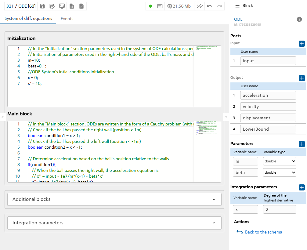
Fig. 1 Block settings

 Two main windows open inside the block:

• Left window for switching between the system of differential equations and events;

• Right window with the variables control panel.

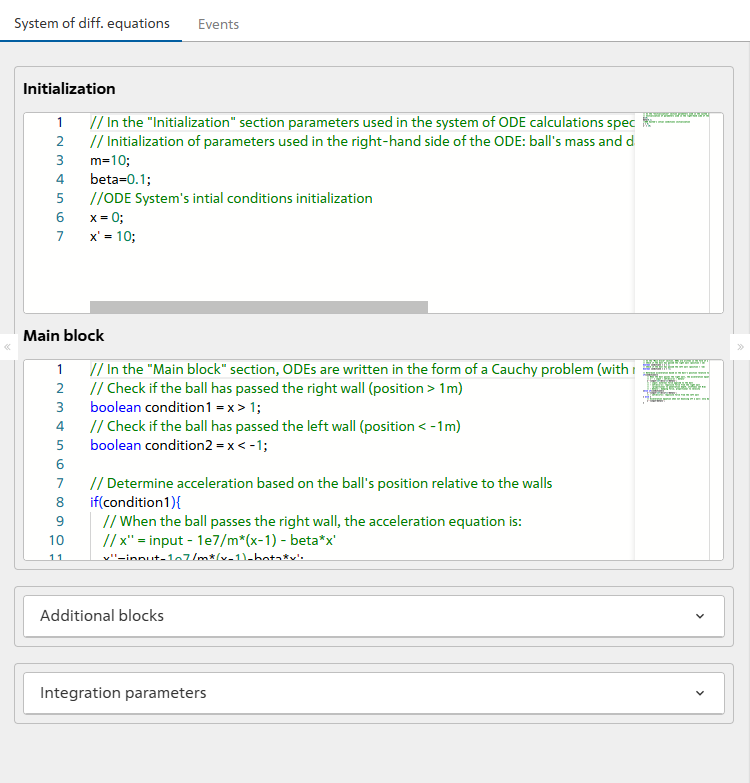
Fig. 2 Left window

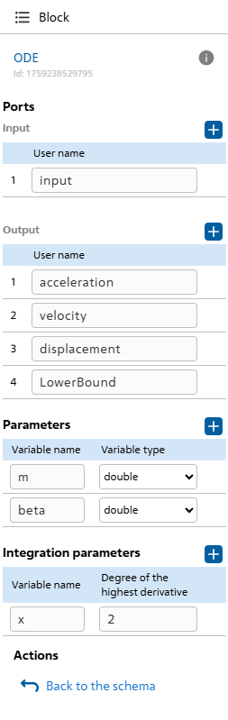
Fig. 3 Right window

 The Differential Equations Section contains the following sections:

• Initialization (see fig. 1);

• Main block (see fig. 1);

• Additional blocks (see fig. 4);

• Integration parameters (see Fig. 5).

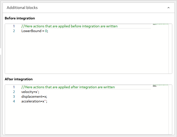
Fig. 4 Additional blocks

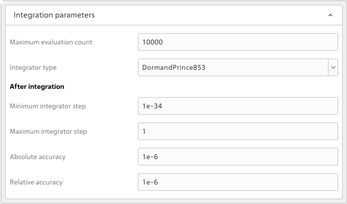
Fig. 5 Integration parameters

Note

To open the sections Additional blocks and Integration parameters, you need to click on their names LMB

 Events Section contains the following sections:

1. Extended event (see Fig. 6);

2. Simple event (see fig. 7).

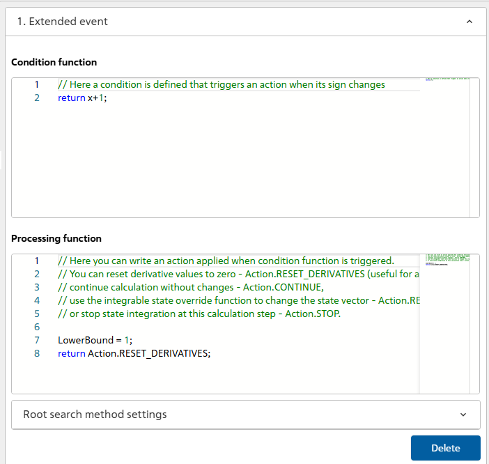
Fig. 6 Extended event

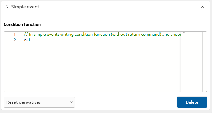
Fig. 7 Simple event

Note

To expand the sections Advanced Event and Simple Event, you need to click on their names LMB

2.  Properties

No

3.  Inputs and outputs

Parameters	Input/Output	Description	Units of measurement	Port type
input	Input	–	–	Automation
acceleration	Output	–	–	Automation
velocity	Output	–	–	Automation
displacement	Output	–	–	Automation
LowerBound	Output	–	–	Automation

In order to see the connection capabilities of the block, you need to go to page Description of block ports

See also

An example of using this block can be found in section Aircraft industry practical guide Development of mathematical model for UAV parachute landing