The procedure for calculating the specific parameters of three-phase PTL models

 This section describes the procedure for calculating the specific (linear) parameters of equivalent circuits for three-phase PTL. This section consists of two parts:

• The first part describes the procedure for calculating the parameters of a PTL in phase coordinates;

• in the second – in symmetrical components.

1.  Parameters of the equivalent circuit of the PTL in phase coordinates

 When calculating the parameters of the equivalent circuit of a PTL in phase coordinates, it is necessary to determine the proper (diagonal elements of the matrix) and mutual (off-diagonal elements of the matrix) linear parameters of the line. The result of calculating the parameters of the PTL are matrices of active resistance \(r\), inductance \(l\), capacitance \(c\) and active conductivity \(g\) with dimensions 3x3, the structure of the obtained matrices using the example of the matrix \(r\) is given in the formula (1):

(1)\[\begin{split}r=\begin{pmatrix} r_{aa} & r_{ab} & r_{ac}\\ r_{ba} & r_{bb} & r_{bc} \\ r_{ca} & r_{cb} & r_{cc} \\ \end{pmatrix},\end{split}\]

where:

 \(r_{aa},r_{bb},r_{cc}\) – own active resistances of phase A, B and C, respectively;

 \(r_{ab},r_{bc},r_{ca}\) – mutual active resistances of phases A and B, B and C, C and A, respectively.

Note

The off-diagonal elements of the matrix must be pairwise equal, since they refer to the same phases: \(r_{ab} = r_{ba}, r_{bc} = r_{cb}, r_{ca} = r_{ac}\). The diagonal elements of the matrix may differ. Thus, to compose each matrix, it is sufficient to calculate 3 diagonal elements and 3 off-diagonal elements for each pair of phases.

1.1.  Calculation of the matrices of active resistance r and inductance l

 Formulas for determining the parameters of the matrices of active resistance \(r\) and inductance \(l\) taking into account the current return circuit through the ground are given in table 1.

Note

To calculate the parameters of the longitudinal resistance matrix of a PTL, various modifications of the Carson formulas are typically used [1]. Table 1 contains the formulas from [2], and one can also use the formulas from [3] (derived for \(f\) = 60 [Hz] in [Ohm/mil], for use in SI units, the coefficients must be recalculated).

Table 1

Parameter	Calculation formula
Conductor’s own active resistance \(r_{ii}\), [Ohm/km]	\(r_{ii}=r_п+r_з=r_п+ \pi^2 \cdot f \cdot 10^{-4}\)
Mutual active resistance of a conductor \(r_{ij}\), [Ohm/km]	\(r_{ij}=r_з=\pi^2 \cdot f \cdot 10^{-4}\)
Self-inductance of a conductor \(l_{ii}\), [H/km]	\(l_{ii}=\frac{\mu_0}{2 \cdot \pi}\cdot ln \frac{D_з}{\rho_{э\hspace{1mm}п}}\)
Mutual inductance of a conductor \(l_{ij}\), [H/km]	\(l_{ij}=\frac{\mu_0}{2 \cdot \pi}\cdot ln \frac{D_з}{d_{ij}}\)

 The following notations are given in table 1:

 \(r_п\) – active phase resistance, [Ohm/km];

 \(r_з\) – active resistance, taking into account the loss of active power in the ground from the current flowing in it, [Ohm/km];

 \(f\) – network frequency, [Hz];

 \(\mu_0=4 \cdot \pi \cdot 10^{-4}\) [H/km] – magnetic constant;

 \( ho_{э\hspace{1mm}п}=k \cdot ho_п\) – equivalent radius of the wire taking into account the surface effect, [m];

 \(k\) is a coefficient that takes into account the surface effect in the conductor: for wires made of non-magnetic material \(k\) = 0.779, for steel-aluminum wires \(k\) = 0.95 [4] [5] [6].

Note

In English-language literature, the value \(GMR= ho_п \cdot e^{-\frac{\mu_п}{4}}\) is used – the geometric mean radius of the wire. When calculating it, the skin effect is also taken into account due to the relative magnetic permeability of the wire material \(\mu_п\), which for non-ferrous metals (copper, aluminum) is taken to be equal to 1. It’s worth noting that the formula given is valid for homogeneous wires. For steel-aluminum wires, GMR can be found in reference literature, for example, in [3]\(^{Appendix A}\).

 \(d_{ij}=\sqrt{(x_i-x_j)^2+(y_i-y_j)^2}\) – distance between the i-th conductor and the j-th conductor, [m] (see Fig. 1);

 \(D_з=\frac{66.4}{\sqrt{f \cdot \lambda}}\) – equivalent depth of the return wire in the ground, [m];

 \(\lambda\) – specific conductivity of the earth, [1/(Ohm·sm)].

Important

When calculating, it is necessary to use the specified units of measurement \(\lambda\).

Note

In calculations, the average conductivity of the earth (wet earth) can be taken to be \(\lambda=10^{-4}\) [1/(Ohm·sm)]. In approximate calculations at \(f\) = 50 [Hz], \(D_з\) = 1000 [m] can then be taken.

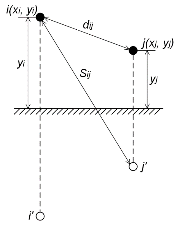
Fig. 1 Determining the distance between conductors and their images

1.2.  Calculation of the capacitance matrices c and active conductivities g

 According to [3], the parameters of the capacitance matrix c can be determined through the inverse matrix of potential coefficients \(p\) using the formula (2):

(2)\[[c_{abc}]=[p_{abc}]^{-1}\]

where:

 \(p_{abc}=\begin{pmatrix} p_{aa} & p_{ab} & p_{ac}\\ p_{ba} & p_{bb} & p_{bc} \\ p_{ca} & p_{cb} & p_{cc} \\ \end{pmatrix}\) – матрица потенциальных коэффициентов;

 \(p_{ii}=\frac{1}{2 \cdot \pi \cdot \epsilon}\cdot ln \frac{2 \cdot y_i}{\rho_{э\hspace{1mm}п}}\) – eigenpotential coefficients;

 \(p_{ii}=\frac{1}{2 \cdot \pi \cdot \epsilon}\cdot ln \frac{S_{ij}}{d_{ij}}\) – mutual potential coefficients;

 \(y_i=\frac{2 \cdot y_{imin}+y_{imax}}{3}\) – средняя высота подвеса i-го проводника, [м] (см. рис. 2);

 \(y_{imax}\) – distance from the attachment point of the i-th conductor on the support to the ground, [m];

 \(y_{imin}\) – minimum distance from the i-th conductor to the ground taking into account the suspension boom, [m];

 \(S_{ij}=\sqrt{(x_i-x_j)^2+(y_i+y_j)^2}\) – distance between the i-th conductor and the image of the j-th conductor, [m] (see Fig. 1);

 \(\epsilon=\epsilon_r \cdot \epsilon_0\) – absolute dielectric constant of the medium;

 \(\epsilon_r\) – relative permittivity of the medium (for air \(\epsilon_r\)=1);

 \(\epsilon_r=8.85 \cdot 10^{-9}\) [F/km] – electric constant.

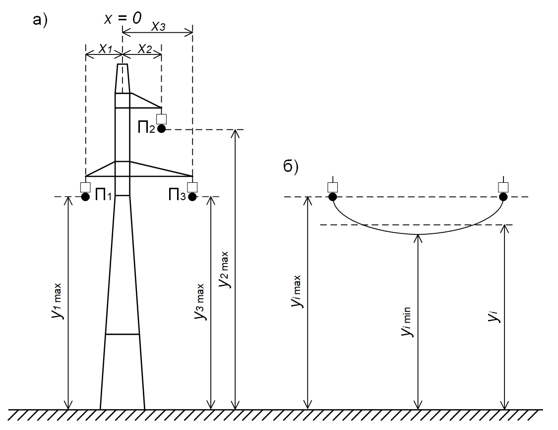
Fig. 2 Location of power transmission line wires on a support
a) determination of wire coordinates;
b) calculation of the average suspension height of the i-th conductor \(y_i\)

Note

In Fig. 2 the \(x_1\) coordinate for wire \(П_1\) will be negative.

Important

The result of calculating the expression (2) will be a matrix of capacitances of the following form (3):

(3)\[\begin{split}c_{abc}=\begin{pmatrix} c_{aa} & -c_{ab} & -c_{ac}\\ -c_{ba} & c_{bb} & -c_{bc} \\ -c_{ca} & -c_{cb} & c_{cc} \\ \end{pmatrix},\end{split}\]

i.e., the off-diagonal elements of the matrix will be negative. This is the format in which the parameters in the Three-phase transmission line (multi-section) block must be specified. When calculating the matrix parameters in any other way, it is necessary to specify in the block a matrix of the specified type, with negative off-diagonal elements.

Note

When using split wires in phase, the calculations for \(r_{ii}, l_{ii}\hspace{1mm} and \hspace{1mm} p_{ii}\) need to be adjusted. Thus, if a phase consists of n identical wires, then the active resistance of the phase is: \(r_п=\frac{r_п^{`}}{n}\), where \(r_п^{`}\) is the resistance of one wire. With increasing n, the equivalent splitting radius of the phase structure increases: \( ho_{э \hspace{1mm} п}=\sqrt[n]{k \cdot ho_п \cdot a^{n-1}}\), where \(a\) is the geometric mean distance between the wires of one phase. According to [7], for simplified calculations one can take \(a\) = (40 – 60) [sm]. A detailed calculation method for \(a\) to take into account the actual distances between the wires of a split phase is given in [3]\(^{chapter 2-5}\).

 Accounting for the active conductivity \(g\) generally depends on the voltage class of the modeled PTL [7] – as a rule, corona losses are taken into account for lines with a voltage class of 330 [kV] and higher. For OL 110 [kV] and 220 [kV] it is permissible not to take \(g\) into account if the diameter of the line wire is equal to or exceeds the minimum specified for reducing corona losses (for OL 110 [kV] – AC-70 (11.8 [mm]), for OL 220 [kV] – AC-240 (21.6 [mm])).

A detailed calculation of active conductivity is a non-trivial task, since corona processes are highly dependent on the OL voltage, atmospheric conditions, and the surface condition of the conductor. A methodology for such calculations is given, for example, in [8]. If, when modeling a PTL, there is no need to take into account corona losses in detail, only the phase conductivities to ground can be taken into account in the calculations. Then the matrix \(g\) will take the form (4):

(4)\[\begin{split}g_{abc}=\begin{pmatrix} g_{aa} & 0 & 0\\ 0 & g_{bb} & 0 \\ 0 & 0 & g_{cc} \\ \end{pmatrix},\end{split}\]

where:

 \(g_{ii}= \frac{\Delta P_ф}{U_{nom}^2}\cdot 10^{-3}\) – specific active conductivity of the phase to ground, [S/km];;

 \(U_{nom}\) – nominal phase voltage, [kV];

 \(\Delta P_ф\) – specific power losses due to corona for one phase, as a rule, are given in reference data (for example, in [9]\(^{table\hspace{1mm} 3.10}\)), [kW/km].

2.  Parameters of the equivalent circuit of the PTL in symmetric coordinates

When calculating the parameters of a PTL equivalent circuit in symmetric coordinates, it is necessary to determine the parameters of the positive and zero sequences of the line. The results of the calculation are the active resistances r_1 and r_0, the inductances l_1 and l_0, and the capacitances c_1 and c_0.

 These parameters can usually be found in reference literature, for example, in [4]. However, if a more accurate calculation is needed, the parameters of the direct and zero sequences can be calculated from the matrices \(r\), \(l\), and \(c\) calculated in step 1.

 According to [3], knowing the parameters of the equivalent circuit of the PTL in phase coordinates, it is possible to determine the values ​​of the parameters in symmetric coordinates using the formula (5):

(5)\[\begin{split}z_{012}=A^{-1} \cdot z_{abc \hspace{1mm} T}\cdot A =\begin{pmatrix} r_{00}+ j\cdot \omega \cdot l_{00} & r_{01}+ j\cdot \omega \cdot l_{01} & r_{02}+ j\cdot \omega \cdot l_{02}\\ r_{10}+ j\cdot \omega \cdot l_{10} & r_{11}+ j\cdot \omega \cdot l_{11} & r_{12}+ j\cdot \omega \cdot l_{12} \\ r_{20}+ j\cdot \omega \cdot l_{20} & r_{21}+ j\cdot \omega \cdot l_{21} & r_{22}+ j\cdot \omega \cdot l_{22} \\ \end{pmatrix}=\begin{pmatrix} z_{00} & z_{01} & z_{02}\\ z_{10} & z_{11} & z_{12} \\ z_{20} & z_{21} & z_{22} \\ \end{pmatrix},\end{split}\]

where:

 \(A=\begin{pmatrix} 1 & 1 & 1\\ 1 & a^2 & a \\ 1 & a & a^2 \\ \end{pmatrix}\) is the matrix of transformation of a three-phase system into a symmetric one, \(a=e^{j \cdot \frac{2 \cdot \pi}{3}}=-0.5 + j \cdot \frac{\sqrt{3}}{2}\) is the operator of a three-phase system;

 \(A^{-1}=\frac{1}{3} \cdot \begin{pmatrix} 1 & 1 & 1\\ 1 & a & a^2 \\ 1 & a^2 & a \\ \end{pmatrix}\) is the matrix inverse of matrix A;

 \(z_{abc}=\begin{pmatrix} r_{aa}+ j\cdot \omega \cdot l_{aa} & r_{ab}+ j\cdot \omega \cdot l_{ab} & r_{ac}+ j\cdot \omega \cdot l_{ac}\\ r_{ba}+ j\cdot \omega \cdot l_{ba} & r_{bb}+ j\cdot \omega \cdot l_{bb} & r_{bc}+ j\cdot \omega \cdot l_{bc} \\ r_{ca}+ j\cdot \omega \cdot l_{ca} & r_{cb}+ j\cdot \omega \cdot l_{cb} & r_{cc}+ j\cdot \omega \cdot l_{cc} \\ \end{pmatrix}\) – матрица продольных сопротивлений в фазных координатах, \(\omega = 2 \cdot \pi \cdot f\) – угловая частота, [рад/с].

 For the transverse conductivity matrix \(y_{abc}=\begin{pmatrix} j\cdot \omega \cdot c_{aa} & j\cdot \omega \cdot c_{ab} & j\cdot \omega \cdot c_{ac}\\ j\cdot \omega \cdot c_{ba} & j\cdot \omega \cdot c_{bb} & j\cdot \omega \cdot c_{bc} \\ j\cdot \omega \cdot c_{ca} & j\cdot \omega \cdot c_{cb} & j\cdot \omega \cdot c_{cc} \\ \end{pmatrix}\) parameters in symmetric coordinates are also determined by the formula (5).

The off-diagonal elements in the (5) formula represent the mutual coupling between sequences. If, according to the calculation results, \(z_{01} = z_{02} = z_{12}\) = 0, then \(z_{00}\) is taken as the zero-sequence resistance, and \(z_{11}\) as the positive-sequence resistance.

 If, according to the calculation results, the matrix \(z_{012}\) has non-zero off-diagonal elements, they must be taken into account when setting the parameters. However, in the case of a transposed line, the mutual impedances between the phases are averaged and become equal. Then the original matrix \(z_{abc}\) can be rewritten in a simplified form with equal self-impedances and equal mutual impedances (6):

(6)\[\begin{split}z_{abc \hspace{1mm}T}=\begin{pmatrix} r_с+ j\cdot \omega \cdot l_с & r_{вз}+ j\cdot \omega \cdot l_{вз} & r_{вз}+ j\cdot \omega \cdot l_{вз}\\ r_{вз}+ j\cdot \omega \cdot l_{вз} & r_с+ j\cdot \omega \cdot l_с & r_{вз}+ j\cdot \omega \cdot l_{вз} \\ r_{вз}+ j\cdot \omega \cdot l_{вз} & r_{вз}+ j\cdot \omega \cdot l_{вз} & r_с+ j\cdot \omega \cdot l_с \\ \end{pmatrix}=\begin{pmatrix} z_с & z_{вз} & z_{вз}\\ z_{вз} & z_с & z_{вз} \\ z_{вз} & z_{вз} & z_с \\ \end{pmatrix},\end{split}\]

where:

 \(z_с=\frac{z_{aa}+z_{bb}+z_{cc}}{3}\) – averaged self-resistance;

 \(z_{вз}=\frac{z_{ab}+z_{bc}+z_{ca}}{3}\) – average mutual resistance.

 By applying the calculations according to the formula (5) to the matrix from the formula (6), we obtain a diagonal matrix of parameters in symmetric coordinates (7):

(7)\[\begin{split}z_{012 \hspace{1mm}T}=\begin{pmatrix} z_{00} & 0 & 0\\ 0 & z_{11} & 0 \\ 0 & 0 & z_{22} \\ \end{pmatrix}=\begin{pmatrix} z_с + 2 \cdot z_{вз} & 0 & 0\\ 0 & z_с - z_{вз} & 0 \\ 0 & 0 & z_с - z_{вз}\\ \end{pmatrix},\end{split}\]

Hint

As can be seen from the formula (7), in the case of a transposed line, it is possible to determine the zero and positive sequence resistance without resorting to matrix calculations.

Important

Formulas (6)- (7) and calculation logic are also applicable for the matrix \(y_{abc}\).

3.  Sources

---

[1]

Carson J. R. Wave propagation in overhead wires with ground return // The Bell System Technical Journal. 1926. Vol. 5, № 4. P. 539–554. DOI: 10.1002/j.1538-7305.1926.tb00122.x.

[2]

Bergen A. R., Vittal V. Power systems analysis. 2nd ed. Upper Saddle River, N.J.: Prentice Hall, 2000. 619 p.

[3] (1,2,3,4,5)

Kersting, W.H. (2012). Distribution System Modeling and Analysis (3rd ed.). CRC Press. https://doi.org/10.1201/b11697.

[4] (1,2)

Guidelines for relay protection. Issue 11. Calculations of short-circuit currents for relay protection and system automation in 110–750 kV networks. – Moscow: Energia, 1979. – 152 p. ill.

[5]

Ulyanov, S.A. Electromagnetic Transient Processes in Electrical Systems. Textbook for Electrical Engineering and Power Engineering Universities and Faculties. Moscow: Energia, 1970.

[6]

Melnikov N.A. Electrical networks and systems. – M.: Energy, 1969. – 456 p. ill.

[7] (1,2)

Gerasimenko A.A., Fedin V.T. Transmission and distribution of electric energy / Gerasimenko A.A., Fedin V.T. - 2nd ed. - Rostov n / D: Phoenix, 2008. - 715 p. - (Higher education).

[8]

RD 34.20.172-74 Guidelines for accounting for corona losses and interference from corona when selecting wires for overhead power transmission lines of alternating current 330 - 750 kV and direct current 800 - 1500 kV. - M., 2009. - 74 p.

[9]

Handbook of electrical network design / edited by D. L. Faibisovich. – 4th edition, revised and enlarged. – Moscow: ENAS, 2012. – 376 p.: ill.