

Asynchronous motor with wound rotor (nonlinear model)#
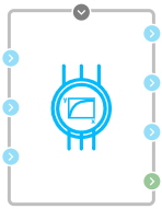
Block appearance in REPEAT VISION#
The Asynchronous motor with wound rotor (nonlinear model) block represents a model of a three-phase electrical machine with a wound rotor, accounting for parameter nonlinearity.
Note
The stator and rotor windings are connected in a star configuration;
The block’s mathematical model is described in the d-q coordinate system, oriented along the rotor flux linkage vector and rotating synchronously with it.
The model is described by the following equations:
where:
\(\psi_{sd}\) – projection of the stator flux linkage onto the d-axis, [Wb];
\(\psi_{sq}\) – projection of the stator flux linkage onto the q-axis, [Wb];
\(i_{sd}\) – projection of the stator current onto the d-axis, [A];
\(i_{sq}\) – projection of the stator current onto the q-axis, [A];
\(R_s\) – active resistance of the stator winding, [Ohm];
\(\omega_e\) – electrical angular frequency, [rad/s].
where:
\(\psi_{rd}\) – projection of the rotor flux linkage onto the d-axis, [Wb];
Note
Since the d-q axis is oriented along the rotor flux linkage, \(\psi_{rq}=0\), and the total rotor flux linkage \(\psi_R=\psi_{rd}\).
\(i_{rd}\) – projection of the rotor current onto the d-axis, [A];
\(i_{rq}\) – projection of the rotor current onto the q-axis, [A];
\(R_r\) – active resistance of the rotor winding, [Ohm];
\(\Delta \omega\) – slip angular frequency, [rad/s] (5):
where:
\(p\) – number of pole pairs;
\(\omega_r\) – rotor angular velocity, [rad/s].
where:
\(L_m\) – mutual inductance between the stator and rotor windings, [H];
\(L_S\) – total stator inductance, [H].
Note
This is the sum of the stator’s self-inductance (leakage inductance) and the mutual inductance between the stator and rotor windings (9):
\(L_R\) – total rotor inductance, [H].
Note
This is the sum of the rotor’s self-inductance (leakage inductance) and the mutual inductance between the stator and rotor windings (10):
mechanics (11):
where:
\(J_Я\) – armature moment of inertia, [\(N\cdot m^2\)];
\(M_{вр}\) – electromagnetic torque on the armature shaft, [\(N\cdot m\)];
\(M_{тр}\) – friction torque, determined by bearing friction and the brush-collector assembly, [\(N\cdot m\)];
\(M_{сн}\) – load torque created by the load on the armature shaft, [\(N\cdot m\)];
Note
This value is supplied to the block externally via the automation port and/or mechanics port.
The torques presented in the equation (11) are calculated using the following formulas:
electromagnetic torque on the armature shaft (12):
friction torque (13):
where \(K_{тр}\) — friction coefficient.
The model implements a nonlinear dependency (14):
where \(i_s\) — amplitude of the stator current vector, defined as (15):
In the block, nonlinearity is specified as an array of numerical values (a table with numerical values for each nonlinearity point). Each point in the array represents a pair of values:
stator current, [A];
mutual inductance between the stator and rotor, [H].
Each point indicates the value of the mutual inductance between the stator and rotor at the current stator current value.
The following requirements apply to the nonlinearity array in this block:
The first point must have the value \(i_s=0\) [A];
There should be no points with the same \(i_s\) current value;
Each subsequent \(i_s\) current value must be greater than the previous one;
The number of \(i_s\) current values must equal the number of \(L_m\) mutual inductance values;
The number of points must be at least two;
Points must not contain negative values.
1. Properties#
Property |
Default Value |
Description |
Units of measurement |
|---|---|---|---|
Pole pairs |
2.0 |
- |
- |
Active resistance of the stator winding |
0.8 |
- |
Ohm |
Stator winding inductance (leakage inductance) |
4.0E-4 |
- |
H |
Rotor winding inductance (leakage inductance) |
0.2 |
- |
Ohm |
Stator inductance |
0.004 |
- |
H |
The points of nonlinearity array – the stator current |
0.0;4.0;8.0;12.0;16.0;200.0 |
Positive values starting from 0 |
А |
The points of nonlinearity array – the mutual inductance |
0.04;0.04;0.04;0.04;0.04;0.04 |
Number of values must equal the number of current values |
H |
Moment of inertia of the rotor |
0.01 |
- |
kg\(\cdot m^2\) |
Rotor friction coefficient |
0.01 |
- |
N\(\cdot m\)/rad/s |
Array of initial conditions [rotor angular frequency (rad/s), rotor angle (rad)] |
0.0;0.0; |
- |
[rad/s; rad] |
2. Inputs and outputs#
Parameters |
Input/Output |
Description |
Units of measurement |
Port type |
|---|---|---|---|---|
External torque |
Input |
Torque value on the shaft from the load |
N\(\cdot\)m |
Automation |
А |
Input |
Start of stator winding phase A |
- |
Electronics |
В |
Input |
Start of stator winding phase B |
- |
Electronics |
С |
Input |
Start of stator winding phase C |
- |
Electronics |
R1 |
Input |
Start of rotor winding phase 1 |
- |
Electronics |
R2 |
Input |
Start of rotor winding phase 1 |
- |
Electronics |
R3 |
Input |
Start of rotor winding phase 1 |
- |
Electronics |
Angular frequency |
Output |
Connects to angular velocity ports of blocks from the Mechanics (Rotational Motion) library |
rad/s |
Angular Velocity |
In order to see the connection capabilities of the block, you need to go to page Description of block ports