

Linear analyzer#
The tool’s functionality solves the problem of providing experimental determination of the frequency dependence of the amplitude ratio (AFC), phase difference (PFC) and group delay (GDT) between the output and input harmonic signals for a complete description of a linear system in the frequency domain.
The Linear analyzer tool is used by clicking on the Linear analyzer button, which is located in the Tools tab of the bottom panel in the General section, Fig. 1:
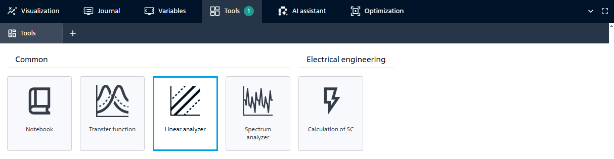
Fig. 1 Linear analyzer#
1. Functional#
The user has several parameters for working with the tool (see Fig. 2 below):
A block is selected from the user’s currently open scheme (drop-down list of blocks);
The input port of the selected block is selected.
A block is selected from the user’s currently open scheme (drop-down list of blocks);
The output port of the selected block is selected.
Limits for linear analysis are selected:
Start frequency and its units of measurement;
End frequency and its units of measurement.
Limits for linear analysis are selected:
Minimum experiment duration, s (Enter a number that must be ≥ 0. Default = 0);
Number of points by frequency (Enter an integer, which must be ≥ 3. Default = 100);
Number of samples per test signal period (Enter an integer, which must be ≥ 2. Default = 10);
Number of test signal periods (Enter an integer, which must be ≥ 1. Default = 10).
Dimensions for graphs must be selected (from the drop-down list):
Amplitude units (
1- dimensionless);Phase units.
There is also an option to turn on/off:
Logarithmic scale;
Compression point.
Parameter hints:
Name |
Hint |
|---|---|
When enabled, test frequencies are adjusted to the project integration step. |
|
Start frequency |
When |
End frequency |
When |
Strictly limited above by the Nyquist criterion (1 / (2 * simulation step)) If the user enters a frequency above this limit, the algorithm forcibly reduces it to the Nyquist frequency to avoid spectrum overlap (aliasing). |
|
Minimum experiment duration, s |
Guaranteed minimum experiment duration for one frequency. |
Number of points by frequency |
|
Number of samples per test signal period |
Minimum number of computed points within one sine-wave period. |
Number of test signal periods |
Number of test signal periods at each frequency. |
Compression point |
A parameter indicating the level of the input or output signal at which the gain of the device is reduced by 1 dB relative to linear mode. Defines the values: OP 1dB — output compression point, IP 1dB — input compression point. |
Important
The final frequency must be greater than the initial frequency;
The specified frequency values must be > 0.
After setting all parameters, the Build graphs button is activated
Note
It is possible to enable the Logarithmic scale (Default: enabled. Default base: 10)
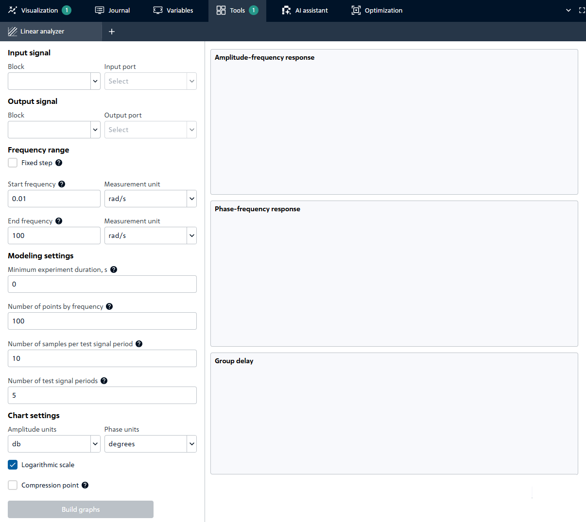
Fig. 2 Setting parameters#
After constructing three graphs (Amplitude-frequency response, Phase-frequency response, Group delay), it becomes possible to work with them in the same way as in the Visualization tab.