Pipe (IH)

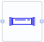
Block appearance in REPEAT VISION

 The unit describes flow of isothermal liquid through the pipe section. The unit takes into account pressure losses during friction against the rough pipe wall.

 Optionally, the unit can take into account compression of isothermal liquid, elastic deformations of pipe walls, inertia of isothermal liquid.

 The pipe can be divided into several sections.

Pressure losses due to friction:

• If the Reynolds number of the flow is less than the upper limit of the Reynolds number for laminar flow, then the pressure losses are calculated by the formula (1) :

(1)\[ \Delta P_{fric} = \frac{\nu \cdot \lambda}{2\cdot D^2\cdot S}\cdot L \ \cdot \dot{m} \]

where:

 \( u\) - kinematic viscosity, [m\(^2\)/s];

 \(\lambda\) - Darcy friction coefficient, which is equal to 64;

 \(L\) – pipe length, [m];

 \(D\) – pipe diameter, [m];

 \(S\) – pipe cross-section area, [m\(^2\)];

 \(\dot{m}\) – mass flow rate of liquid, [kg/s].

• If Reynolds number of flow is greater than the lower limit of the Reynolds number for turbulent flow, then pressure losses are calculated by the formula (2) :

(2)\[ \Delta P_{fric} = \frac{f}{2\cdot \rho \cdot S^2} \cdot \frac{L}{D} \cdot \mid \dot{m} \mid \cdot \dot{m} \]

where:

 \(f = \{-1.8 \cdot \ log_{10}[\frac{6.9}{Re} + (\frac{\varepsilon}{3.7\cdot D_h})^{1.11}] \}^{-2}\);

 \( ho\) – liquid density, [kg/m\(^3\)];

 \(S\) – pipe cross-section area, [m\(^2\)];

 \(L\) – pipe length, [m];

 \(D\) – pipe diameter, [m];

 \(\dot{m}\) – mass flow rate of liquid, [kg/s];

 \(Re\) – Reynolds number;

 \(\varepsilon\) - pipe roughness;

 \(D_h\) – hydraulic diameter of the pipe, [m].

• If the Reynolds number corresponds to a transient process, then the resistance coefficient is linear interpolation between the boundary points of the turbulent and laminar flow condition.

Mass conservation principle:

• If liquid is incompressible, then flowrate at the pipeline inlet and outlet is the same. If compressed liquid mode is selected, then each pipe segment is divided into three parts - two pipes connected by a capacitive unit. The mass conservation principle in a capacitive unit is determined by the ratio:

(3)\[ \dot{m_A} + \dot{m_B} = \dot{P_n} \cdot \frac{\Delta \rho_n}{\Delta P_n}\ \cdot V \cdot \dot{m_A} \]

where:

 \(\dot{m_B}\) – mass flow rate of liquid in the “left” pipe, [kg/s];

 \(\dot{m_B}\) – mass flow rate of liquid in the “right” pipe, [kg/s];

 \(P_n\) – pressure in the capacitive unit, [Pa];

 \( ho_n\) – density of liquid in the capacitive unit, [kg/m\(^3\)];

 \(V\) – pipe segment volume, [m\(^3\)].

• If deformations of pipeline walls are taken into account, then the term associated with the volumetric expansion is added to the mass conservation principle: (4) :

(4)\[ \dot{m_A} + \dot{m_B} = \dot{P_n}\cdot \frac{\Delta \rho_n}{\Delta P_n}\ \cdot V + \rho_n \cdot \dot{V} \]

Momentum conservation law:

 The total pressure differential between pipe ends is determined by friction losses and elevation differences (5) :

(5)\[ \Delta P = \Delta P_{fric} + \rho \cdot \Delta z \cdot g \]

 \(P_{fric}\) - friction pressure losses, [Pa];

 \( ho\) – liquid density, [kg/m\(^3\)];

 \(\Delta z\) - difference of elevations, [m];

 \(g\) – gravity acceleration, [m/s\(^2\)].

 If liquid inertia is taken into account, then the total pressure differential is determined by the formula (6) :

(6)\[ \Delta P = \Delta P_{fric} + \rho \cdot \Delta z \cdot g + \ddot{m} \cdot \frac{L}{2\cdot S} \]

 \(L\) – pipe length, [m];

 \(S\) – pipe cross-section area, [m\(^2\)].

Pipe specifications

 If deformable walls of the pipeline are selected, then the volumetric expansion of the pipe is calculated by the formula (7) :

(7)\[ \dot{V} = \frac{\pi}{2}\cdot D \cdot L\cdot \frac{D(p)-D}{\tau} \]

where:

 \(\dot{V}\) – volumetric expansion, [m\(^3\)];

 \(L\) – pipe length, [m];

 \(D(P)\) - pipeline diameter depending on pressure, [m];

 \(D\) – pipeline diameter at the previous integration step, [m];

 \( au\) – volumetric expansion time constant.

 Change in pipe diameter, as well as volumetric expansion, is limited by the time constant of volumetric expansion.

 Pipe diameter depends on the static pressure in the pipe segment (8):

(8)\[D(P) = D_n \cdot(1 + \epsilon_{hoop})\]

where:

 \(\epsilon_{hoop} = \frac{P\cdot D_n}{2\cdot E \cdot h} \cdot [1 - \frac{\nu}{2}]\)

 \(P\) – static pressure inside the pipe, [Pa];

 \(D_n\) – nominal pipe diameter, [m];

 \(E\) - Young’s modulus of the pipe wall;

 \(h\) – pipe wall thickness, [m];

 \( u\) - Poisson’s ratio.

1.  Properties

Property	Default value	Description	Units of measurement
Fluid dynamic compressibility	Off	-	-
Fluid inertia, available when Fluid dynamic compressibilit - On	Off	-	-
Number of segments, available when Fluid dynamic compressibilit - On	1	-	-
Pipe length	5	-	m
Pipe diameter	0.1	-	m
Elevation gain from port A to port B	0	-	m
Gravitational acceleration	9.81	-	м/с\(^2\)
Internal surface absolute roughness	15e-6	-	m
Laminar flow upper Reynolds number limit	2000	-	-
Turbulent flow lower Reynolds number limit	4000	-	-
Pipe wall is rigid?, available when Fluid dynamic compressibility - On	On	-	-
Pipe wall thickness, available when Fluid dynamic compressibility - On and Pipe wall is rigid? - Off	0.05	-	m
Pipe wall thickness, available when Fluid dynamic compressibility - On and Pipe wall is rigid? - Off	6.9e10	-	Pa
Pipe wall thickness, available when Fluid dynamic compressibility - On and Pipe wall is rigid? - Off	0.33	-	-
Pipe wall thickness, available when Fluid dynamic compressibility - On and Pipe wall is rigid? - Off	0.01	-	s
Initial liquid pressure, available when Fluid dynamic compressibility - On	0	-	Pa
Initial mass flow rate, available when Fluid dynamic compressibility - On and Fluid inertia - On	0	-	kg/s

2.  Inputs and outputs

Parameters	Input/Output	Description	Units of measurement	Port type
Input	Input	-	-	Isothermal hydraulics
Output	Output	-	-	Isothermal hydraulics

In order to see the connection capabilities of the block, you need to go to page Description of block ports

3.  Примеры использования

Для быстрого ознакомления с данным блоком откройте один из следующих ДЕМО-примеров:

1. [DEMO] Трубопровод между двумя резервуарами

2. [DEMO] Трубопровод с местным сопротивлением

3. [DEMO] Модель нестационарного течения в системе водоснабжения

4. [DEMO] Поиск требуемого расхода в трубопроводной системе

С примером использования данного блока можно ознакомиться:

• В уроке Pipeline between two reservoirs

• В практическом руководстве Determining the required water flow rate in a pipeline system