

Tire (Magic formula)#

Block appearance in REPEAT VISION#
The Tire (Magic formula) block models a car wheel, including:
conversion of rotation into translational motion;
longitudinal interaction of the tire with the road (Magic formula);
(optional) rolling resistance;
(optional) tire elasticity and damping;
(optional) wheel inertia.
The block implements the interaction of the tire with the road surface using the empirical model Magic formula (Paseyka formula) [1] for calculating the longitudinal force, Fig. 1:
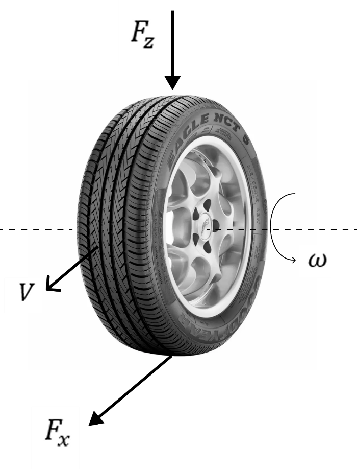
Fig. 1 Forces acting on the wheel (longitudinal dynamics)#
The equation of the wheel (1):
where:
\(\omega\) – angular velocity of the axis, [rad/s];
\(R\) – wheel radius, [m].
Slip calculation (in r.u.) (2) :
where:
\(\nu_{wheel}\) – longitudinal speed of the wheel circumference (tread), [m/s];
\(\nu_{hub}\) – longitudinal speed of the wheel hub, [m/s];
\(\nu_{hub_{smooth}}\) - smoothed longitudinal speed of the wheel hub, the lower speed threshold is equal to the value of the parameter Lower boundary of slip denominator, [m/s], (To prevent division by zero);
\(saturation\) – smoothed constraint with the range [\(k_{min},k_{max}\)], the width of the transition zone for the smoothed constraint depends on the parameter Velocity threshold of slip;
\(k_{min}\) – parameter Minimum valid wheel slip, r.u.;
\(k_{max}\) – parameter Maximum valid wheel slip, r.u.
After calculating the slip, the longitudinal force is determined through the stationary characteristic of the tire (3):
where:
\(F_x\) - longitudinal force, [N];
\(F_{z_{input}}\) - vertical load, [N];
\(k\) - longitudinal slip, %.
The function \(f(k, F_{z_{input}})\) describes the nonlinear dependence of force on slip:
for small \(k\), the force grows almost linearly;
at \(k=k_{peak}\) — the maximum is reached, where \(k_{peak}\) is the slippage that occurs at the maximum longitudinal force \(F_{x_{peak}}\) and the nominal load \(F_{z_{rated}}\);
for large \(k\), the force decreases (slippage).
The model uses parameterization through:
maximum longitudinal force \(F_{x_{peak}}\), [N];
corresponding sliding \(k_{peak}\), %;
nominal vertical load \(F_{z_{rated}}\), [N].
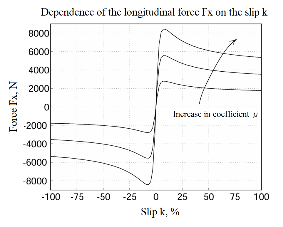
Fig. 2 Typical characteristic Fx(k)#
Paying attention to Fig. 2 above, it is worth noting that the effective adhesion coefficient μ is not an explicit parameter of the model and is not involved in the calculations during the modeling process. It can be used in the parameterization stage to specify the maximum longitudinal force \(F_{x_{peak}}\) via the nominal vertical load \(F_{z_{rated}}\) (4) :
Important
It should be taken into account that this definition corresponds to the nominal load and does not reflect the dependence of the force on the current vertical load and slip, which is taken into account within the Magic formula approximation.
Based on \(F_{x_{peak}}\), \(F_{z_{rated}}\), \(k_{peak}\), the coefficients of the Paseyka formula are calculated, after which the force is defined as (5) :
where \(B_x,C_x,D_{x_{N}},E_x\) are the Magic formula coefficients.
Magic formula coefficients (6):
where:
\(a_1,a_2,a_3,a_4,a_5,a_6,a_7,a_8\) - empirical coefficients of the bus relative to which the parameters are scaled;
\(F_z=\frac{F_{z_{input}}}{F_{z,sf}}\) – relative vertical load.
When parameterizing the model with respect to the peak longitudinal force and slip, scaling of the parameters is introduced (7) :
where \(F_{z_0},F_{x_0},k_0\) are the parameters of the bus relative to which the parameters are scaled.
The longitudinal force \(F_x\), calculated using the Magic formula, is transferred to the translational port and participates in the equation of motion of the Veh.
Optionally, the translational force of the wheel can also be formed taking into account:
rolling resistance \(F_{roll}\);
longitudinal elastic and damping forces \(F_{spring},F_{damp}\).
Rolling resistance equation (8) :
where:
\(k_{roll}\) – rolling coefficient;
\(\nu_{thr}\) – speed limit for calculating the rolling force, [m/s].
Equation of longitudinal dynamics forces (9):
\(x_{wheel}\) - longitudinal displacement of the wheel, [m];
\(k_{stiff}\) – longitudinal stiffness coefficient, [N/m];
\(k_{damp}\) - longitudinal damping coefficient, [N\(\cdot\)s/m].
only longitudinal dynamics are taken into account;
no lateral forces;
there is no combined sliding.
1. Properties#
Property |
Default Value |
Description |
Units of measurement |
|---|---|---|---|
Rated vertical load |
3000.0 |
- |
N |
Peak longitudinal force |
3500.0 |
- |
N |
Slip at peak force at rated load |
10.0 |
- |
% |
Wheel radius |
0.3 |
- |
m |
Rolling resistance model: |
None |
- |
- |
Rolling coefficient |
0.012 |
Available, when |
- |
Velocity threshold of rolling resistance |
0.01 |
Available, when |
m/s |
Off |
- |
- |
|
Longitudinal stiffness |
1000000.0 |
Available, when |
N/m |
Longitudinal damping |
1000.0 |
Available, when |
N/(m/s) |
Off |
- |
- |
|
Inertia |
0.75 |
Available, when |
kg \(\cdot\) m\(^2\) |
Initial angular velocity |
0.0 |
Available, when |
rad/s |
Off |
- |
- |
|
0.1 |
Available, when |
m/s |
|
1.0 |
Available, when |
m/s |
|
-1.5 |
Available, when |
- |
|
1.5 |
Available, when |
- |
2. Inputs and outputs#
Parameters |
Input/Output |
Description |
Units of measurement |
Port type |
|---|---|---|---|---|
Normal force \(F_{z}\) |
Input |
- |
N |
Automation |
Axle |
Input |
- |
- |
Rotational motion |
Slip |
Output |
- |
% |
Automation |
Hub |
Output |
- |
- |
Translational motion |
In order to see the connection capabilities of the block, you need to go to page Description of block ports