Visualization

The visualization pop-up panel is designed to display simulation data graphically when a user task is performed. This panel is opened with a button on the canvas (see Fig. 1) or on the bottom panel on the left (see Fig. 2), as indicated by the arrows below.

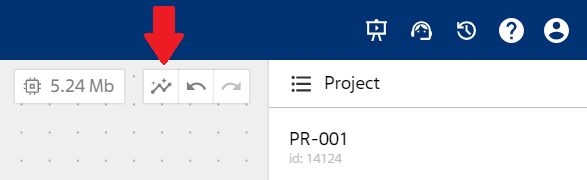
Fig. 1 «Visualization» button in the upper right corner of the canvas

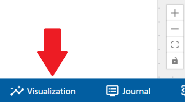
Fig. 2 Duplicating «Visualization» icon on the left on the bottom panel under the canvas

To draw graphs on the visualization panel, click the icon to expand the Block parameter field (see Fig. 3). In this way, you can call up several visualizations for simultaneous demonstrations. Parameter selection to visualize can be done by adding it from the pull-down list, by clicking on “Block parameters, Y-axis” (see Fig. 4) or by selecting the required block on the operating scheme (the block will be indicated by a blue frame, see Fig. 5) and selecting the required parameter in the pull-down list (in this case the pull-down list will be reduced to parameters presented by the selected block) (see Fig. 4, Fig. 5 or Fig. 6).

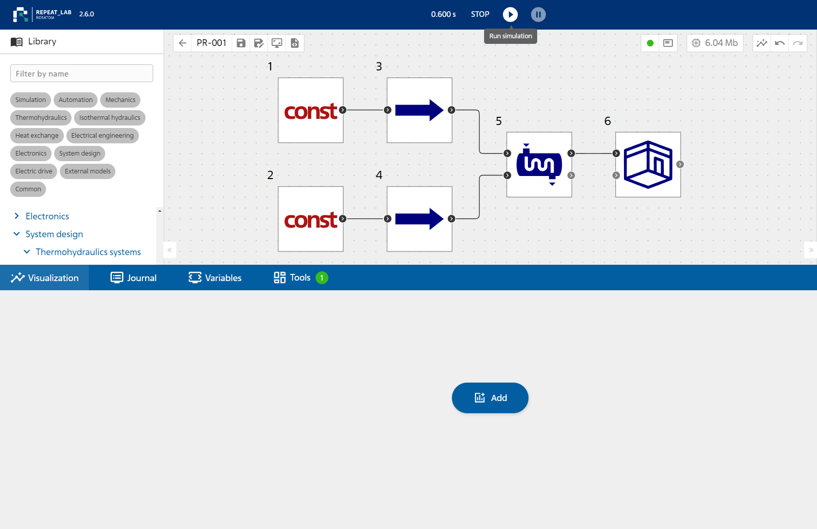
Fig. 3 Calling up block parameters for visualization

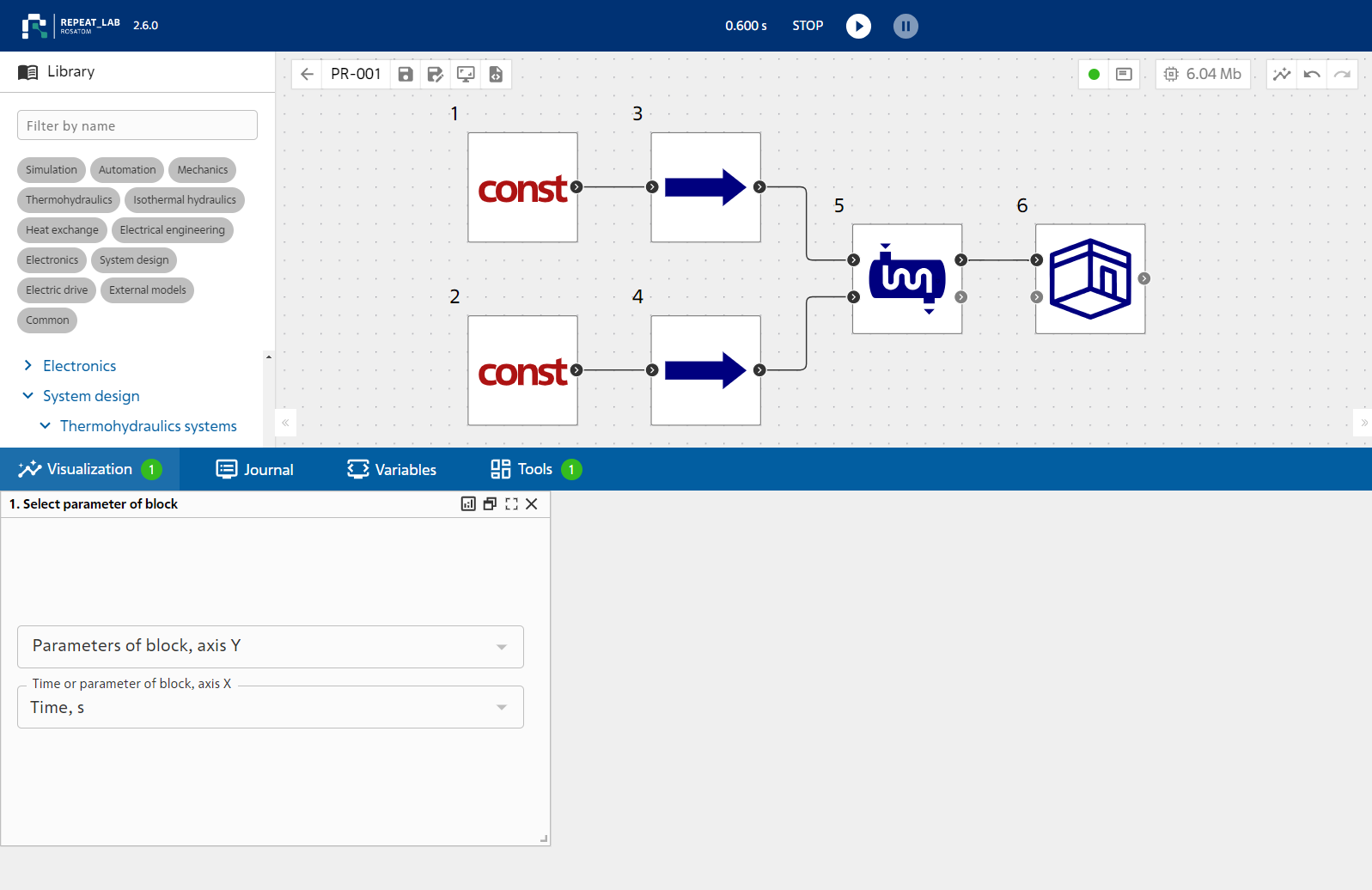
Fig. 4 Example of calling up the parameter drop-down list

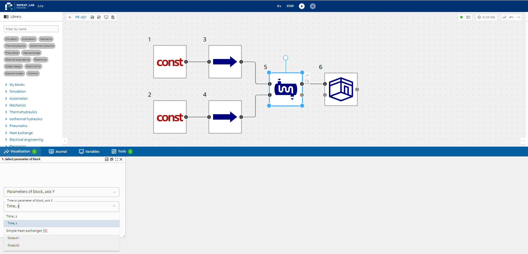
Fig. 5 Example of selection of parameters for selected block №5

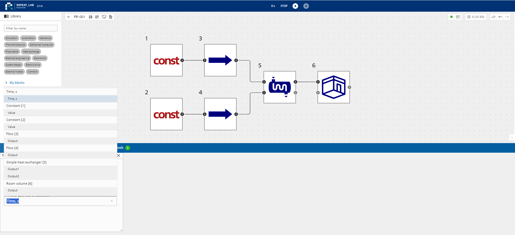
Fig. 6 Variable selector for visualization in drop-down list for all circuit blocks

The search field uses a name mask filter to quickly search large lists.

The following is an example of an ongoing visualization process at the output of the rectangular pulse generator and relaxation circuit (see Fig. 7, block №1 and block №2). Telemetry of the running visualization for each graph can be downloaded to the local computing resource as a CSV file.

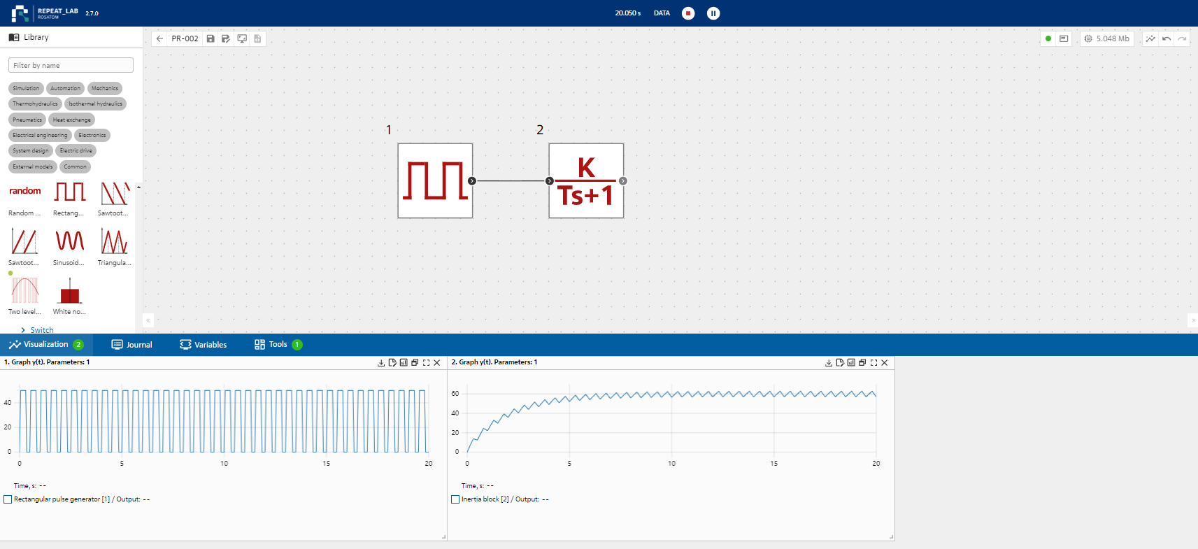
Fig. 7 Example of visualization at output of rectangular pulse generator and relaxation circuit

In order to open the visualization area in full screen, it is necessary to click on the button , located on the center panel on the right.

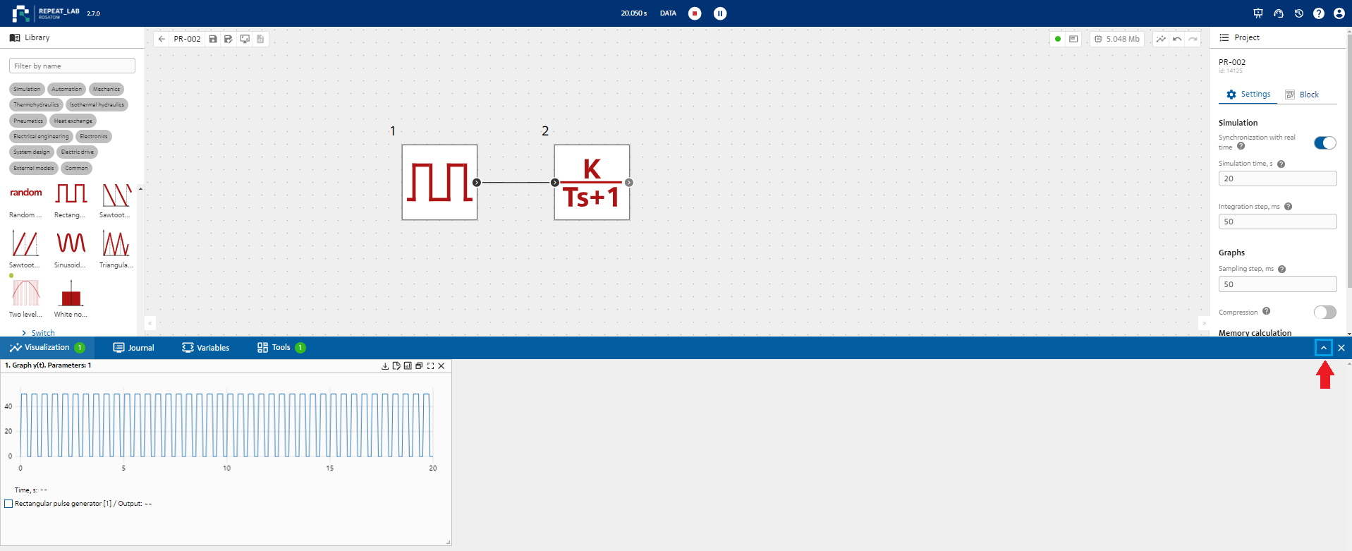
Fig. 8 Open the visualization area to full screen

After clicking on the button, the visualization area will open to full screen.

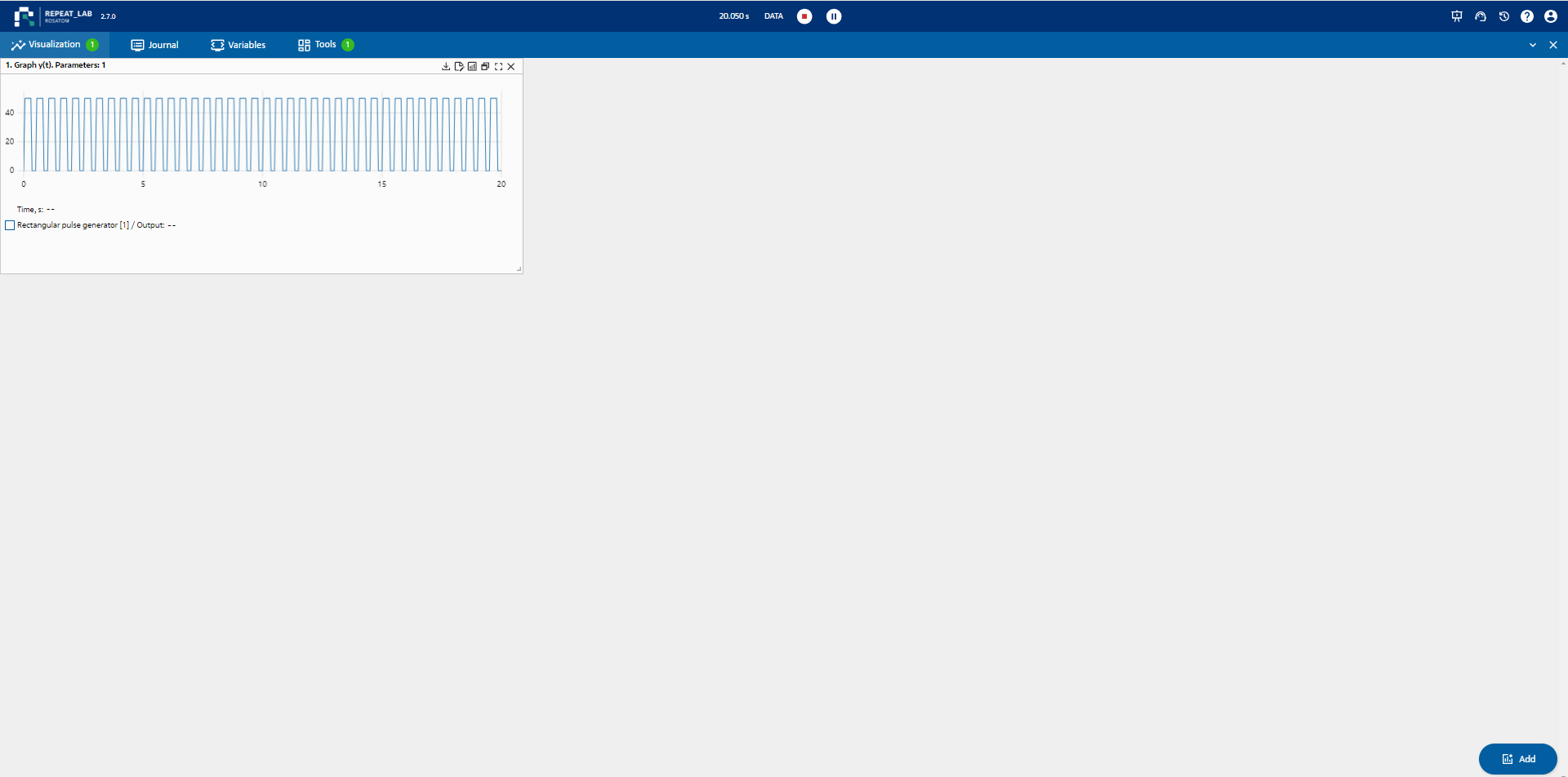
Fig. 9 Example of opening a full-screen visualization area

In order to collapse the visualization area to its original view, click on the button located in the upper panel on the right.

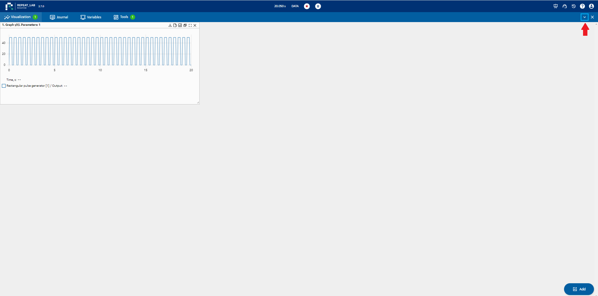
Fig. 10 Example of collapsing the visualization area back to its original form

Also in the visualization area, where the constructed graph is displayed, it is possible to download CSV file (comma-separated data file), which can be created and edited in Excel and easily transferred from one program to another. In order to do this it is necessary to click on button (“Download CSV”), located on the upper panel on the right, after which the file will start downloading to the used computer.

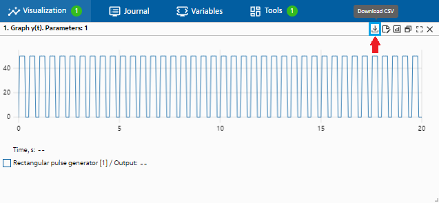
Fig. 11 Downloading CSV file

If it is necessary to edit the graph in terms of its construction according to block parameters, time along the axes, click on the button (“Edit”) located on the upper panel on the right.

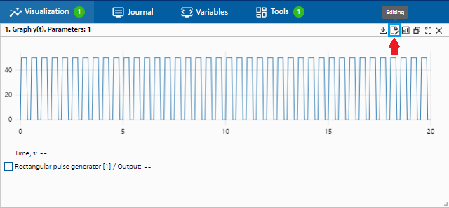
Fig. 12 Editing of graph by axes

After making changes to at least one of axes (lines 1 and 2) or in case if no changes are required, it is necessary to confirm the editing by clicking on the button (“Edit”),which appeared after clicking on the button .

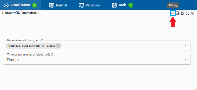
Fig. 13 Confirmation of editing

In order to open the graph editing window it is necessary to click on the button (“Open Graph Editor”)

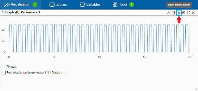
Fig. 14 Editing of graph

The following editing options will appear in the window that opens.

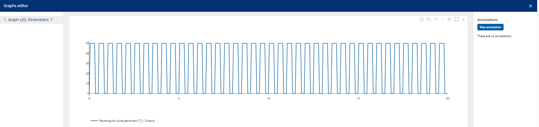
Fig. 15 Graph editing window

In order to enter annotations, it is necessary to click on the “Add” button on the right panel. Then, holding down the left mouse button, it is necessary to move the “test” annotation to the desired place. In order to rename the annotation, click on the “test” inscription located on the graph and enter the required name, which is duplicated in the right panel.

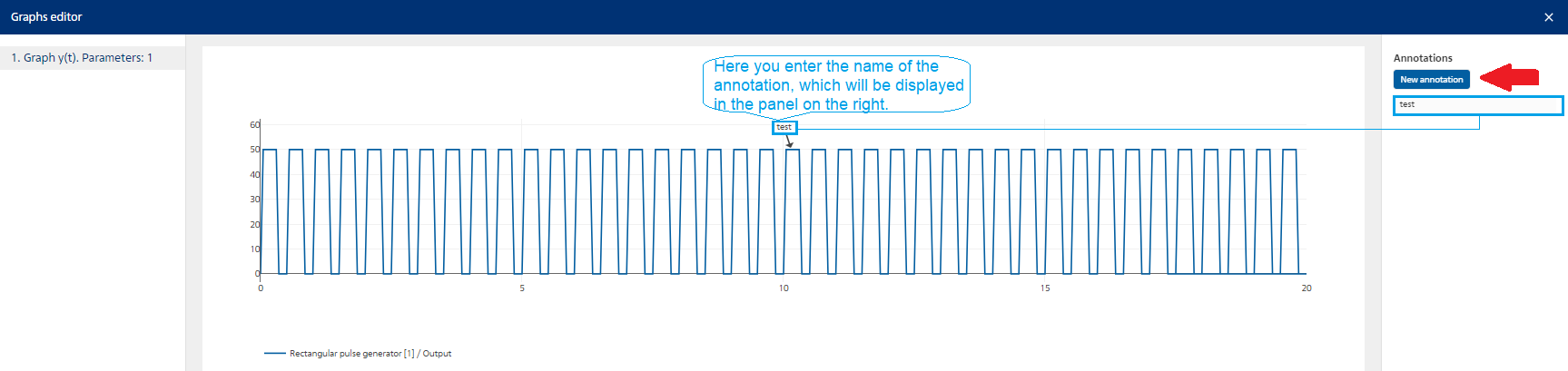
Fig. 16 Adding annotations

Annotations are deleted by clicking on the button , that appears when hovering over the annotation name in the right pane.

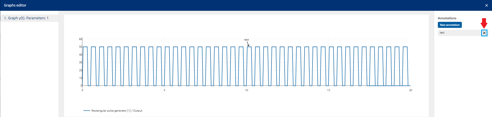
Fig. 17 Deletion of annotations

In order to return to the original display of the graph, click on the button (“Reset displays to default values”) located on the top panel.

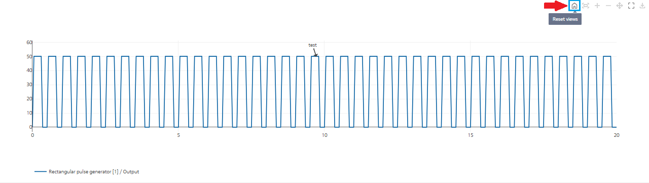
Fig. 18 Resetting Displays to Default Values

In order to adjust the scale of the graph to the viewing area, click on the button (“Automatic scaling”) located on the top panel.

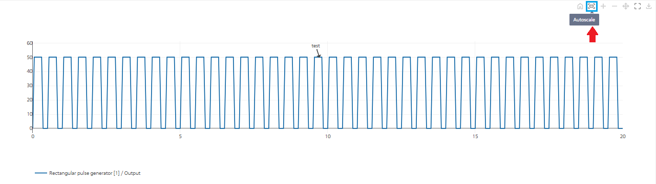
Fig. 19 Automatic scaling

In order to increase the scale of the graph, click on the button (“Increase”) located on the upper panel.

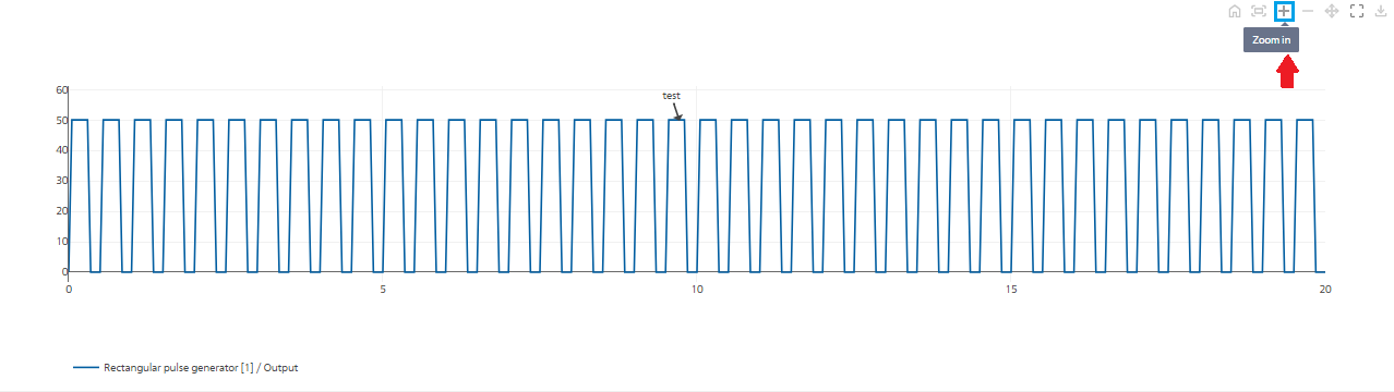
Fig. 20 Scaling-up

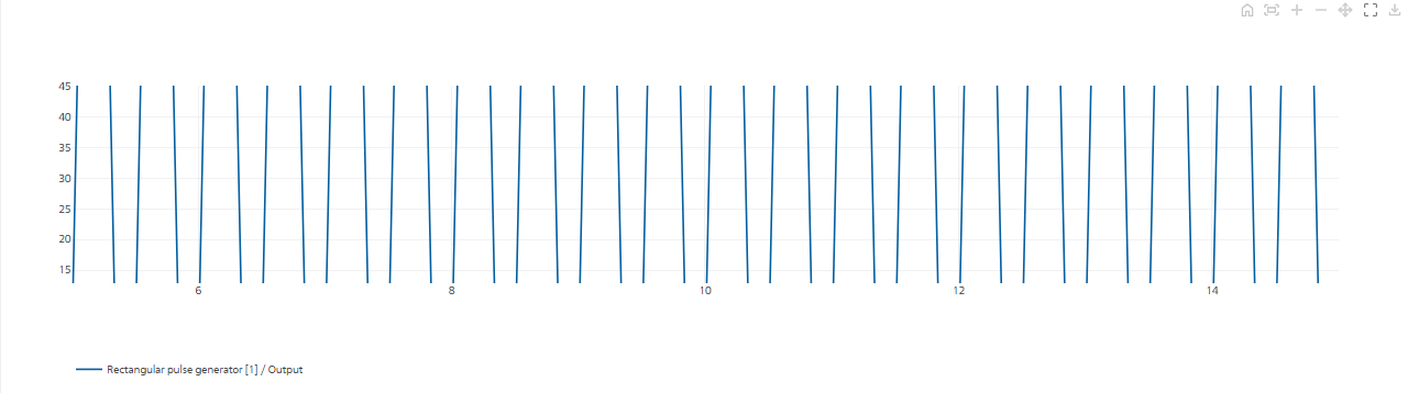
Fig. 21 Graph after scaling-up

It is also possible to scale up the graph by pointing the mouse on the necessary fragment and, holding down the left mouse button, select the necessary area for viewing. This is called “Scaling up mode in the selected area” and is indicated by the following symbol in the top right panel. The larger the selection, the larger the scale.

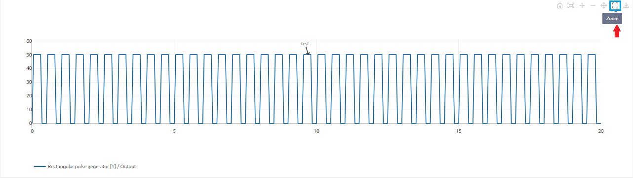
Fig. 22 Scaling up mode in the selected area

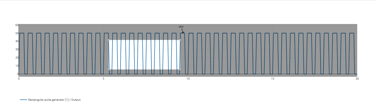
Fig. 23 Area selection

After we stop pressing the left mouse button to enlarge the selection area, the selection will be scaled.

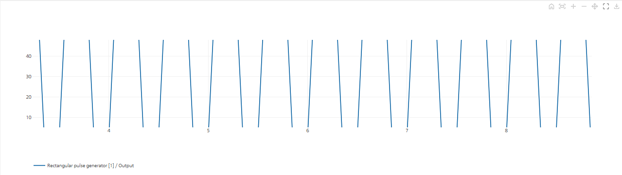
Fig. 24 Scaling up with the mouse

In order to scale down the graph, it is necessary to click on the button (“Reduce”) located in the upper panel.

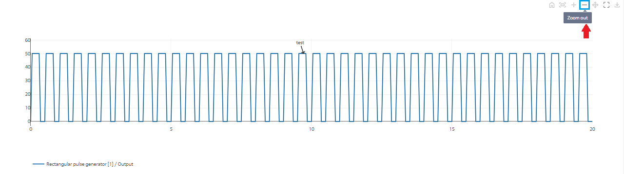
Fig. 25 Scaling down

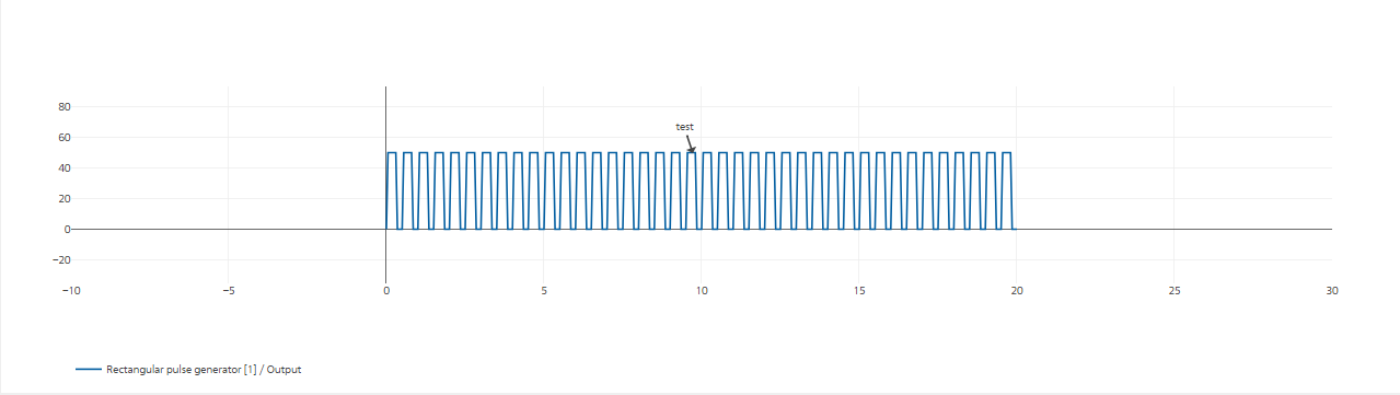
Fig. 26 Example of scaled down graph

The cursor with this symbol is used to move through the graph. In order to move the cursor on the chart, click the left mouse button and move it in the desired direction. It is necessary to stop clicking the left mouse button when the movement is complete.

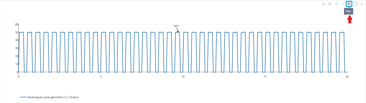
Fig. 27 Graph movement mode

In order to save the graph in SVG format, click on the button (“Save graph in SVG format”) located in the upper panel on the right.

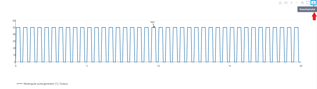
Fig. 28 Saving the graph in SVG format

After clicking, the file will be downloaded to the computer used. In order to exit “Graphs editor” click on the button , located on the upper panel on the right

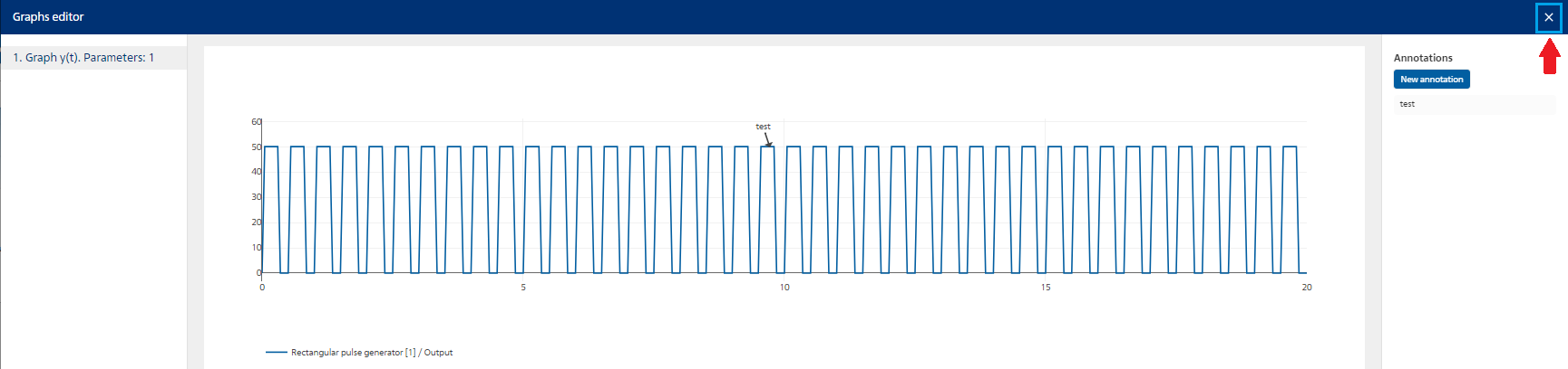
Fig. 29 Exit from graphs editor