Orifice (P)

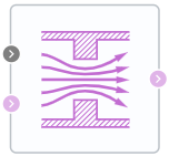
Block appearance in REPEAT VISION

 The Orifice (P) unit simulates flow through a local constraint with a constant or variable hole area. The opening area is parameterized either linearly or using a lookup table.

 The unit retains mass so that (1):

(1)\[ \dot m_{A}\:+\:\dot m_{B}\:=\:\rho_A\:\cdot\:\nu_{A}\:\cdot\:A_{A}\:+\: \rho_B\:\cdot\:\nu_{B}\:\cdot\:A_{B}\:=\:0 \]

 This mass balance implies that the velocity increases when the area decreases and decreases when the flow is discharged over a larger area. In accordance with Bernoulli’s principle, this change in velocity results in a region of lower bore pressure and higher expansion are pressure. The resulting increase in pressure, which is called pressure recovery, depends on the loss coefficient at restoring pressure and the ratio of the areas of the hole and port.

Mass flow calculation

 The unit calculates the mass flow rate as follows (2):

(2)\[ \dot m=C_d \cdot S_r \cdot \sqrt {\frac{2 \cdot \gamma}{\gamma - 1}\cdot p_{in} \cdot \rho_{in} \cdot (\frac{p_{out}}{p_{in}})^{\frac {2}{\gamma}}\cdot(\frac{1-(\frac{p_{out}}{p_{in}})^{\frac {\gamma-1}{\gamma}}}{1-(\frac{S_R}{S})^2\cdot(\frac{p_{out}}{p_{in}})^{\frac {2}{\gamma}}})}\]

where:

 \(C_d\) – discharge coefficient;

 \(S_r\) – area of the hole, [m\(^2\)];

 S — cross-sectional area of ports A and B, [m\(^2\)];

 \( ho\) – gas density, [kg/m\(^3\)];

 p - gas pressure, [Pa];

 \(\gamma\) - adiabatic exponent.

 Linearization of the equation for \(\frac{p_{out}}{p_{in}}\)>B\(_{lam}\) (3):

(3)\[ \dot m=C_d \cdot S_r \cdot \sqrt {\frac{2 \cdot \gamma}{\gamma - 1}\cdot p_{avg}^{\frac {2 - \gamma}{\gamma}} \cdot \rho_{avg} \cdot B_{lam}^{\frac {2}{\gamma}}\cdot(\frac{1- B_{lam}^{\frac {\gamma - 1}{\gamma}}}{1-(\frac{S_r}{S})^2\cdot B_{lam}^{\frac {2}{\gamma}}}})\cdot (\frac {p_{in}^{\frac {\gamma - 1}{\gamma}}-p_{out}^{\frac {\gamma - 1}{\gamma}}}{1-B_{lam}^{\frac {\gamma - 1}{\gamma}}})\]

 When the pressure ratio is less than the ratio \(\frac{p_{out}}{p_{in}}\) < \((\frac{2}{\gamma +1})^\frac {\gamma}{\gamma-1}\) the equation assumes (4):

(4)\[ \dot m=C_d \cdot S_r \cdot \sqrt {\frac{2 \cdot \gamma}{\gamma + 1}\cdot p_{in} \cdot \rho_{in} \cdot (\frac{1}{(\frac{\gamma +1}{2})^{\frac{2}{\gamma -1}}-(\frac{S_r}{S})^2}})\]

Energy conservation law (5):

(5)\[ {\phi}_{A}+{\phi}_{B}=0 \]

where:

 \(\phi_А\) - energy flow at the input, [W];

 \(\phi_В\) - energy flow at the output, [W].

1.  Properties

Property	Default Value	Description	Units of measurement
Orifice type: Variable; Constant	Variable	-	-
Port area	0.001	-	m\(^2\)
Orifice area	1.0E-4	-	m\(^2\)
Orifice area vector	{1.0E-9; 2.0352E-7; 4.0736E-5; 1.1438E-4; 3.4356E-4;}	-	m\(^2\)
Discharge coefficient	0.64	-	-
Laminar flow pressure ratio	0.999	-	-

2.  Inputs and outputs

Parameters	Input/Output	Description	Units of measurement	Port type
Auto, available when Orifice type - Variable	Input	-	-	Automation
Input	Input	-	-	Pneumatics
Output	Output	-	-	Pneumatics

In order to see the connection capabilities of the block, you need to go to page Description of block ports

3.  Examples of use

 Examples of using this block can be found in the following sections:

• Tutorials;

• How-to guides;

• Description of Demo.

Tutorials

Library	Tutorial name
Pneumatics	Gas outflow to a cylinder through a tube with a narrowing

How-to guides

Section	Guide name
Machine learning approximation	Approximation model of gas flow through a nozzle
Solving optimization tasks	Maximizing gas production rate in the gas well cluster collection system