Approximation model of gas flow through a nozzle

This practical guide presents the steps for implementing a machine learning model designed to approximate the process of gas flow through a nozzle, and also presents a method for using the ML model on the REPEAT VISION platform.

Note

If you do not have basic knowledge of the REPEAT VISION Pneumatics library, please review the introductory tutorial before continuing with this tutorial.

1.  Modeling gas flow in a simple pipeline system

To focus on the process of creating a machine learning model, it is necessary to prepare a model of a simple piping system to calculate gas flow through a nozzle. A diagram of the required project is shown in the figure below.

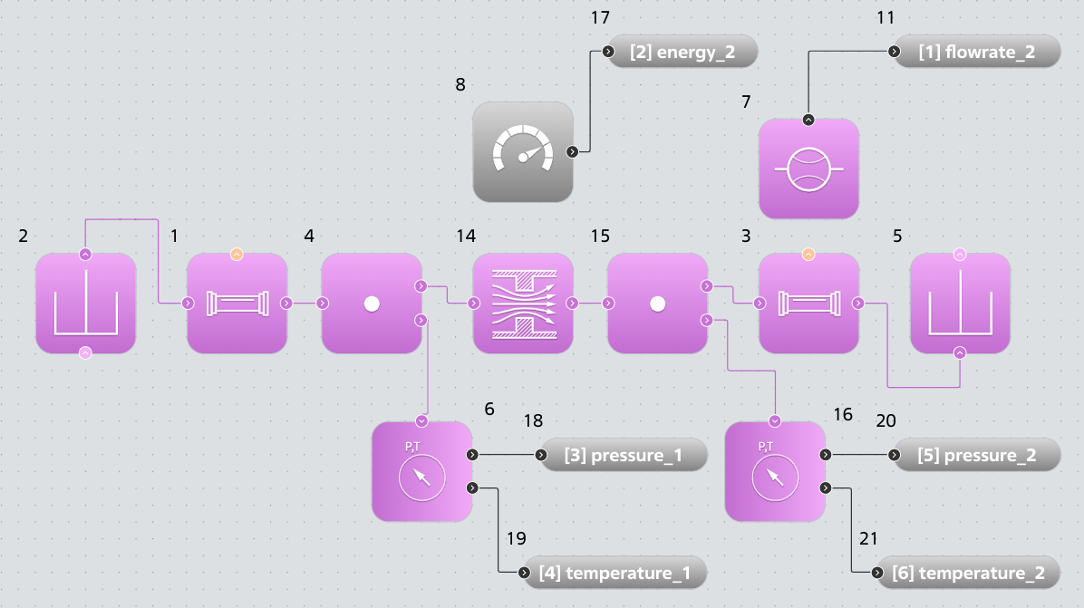
A simple piping system for simulating gas flow through a nozzle.

The project shown above allows us to investigate the change in gas mass flow and energy flow through the nozzle - block No. 14 Approximation model (P) - when changing the parameters given in the table below.

Parameter	Parameter type	Global variable name	Meaning	Applies to block
Tank pressure	Boundary condition \([Pa]\)	PRESS	7.5e6	Block №2 Reservoir (P)
Temperature	Boundary condition \([^{\circ}C]\)	TEMP	20.0	Reservoir (P) №2 and №5, as well as Pipe (P) №1 and №3

Blocks Reservoir (P) №2 and №5 have the following settings:

Property	Block №2	Block №5
Gauge pressure \([Pa]\)	PRESS	5e6
Temperature \([^{\circ}C]\)	TEMP	TEMP
Port cross-sectional area \([m^2]\)	0.2	0.2

Blocks Pipe (P) №1 and №3 contain the following settings:

Property	Meaning
Gas compressibility	Not taken into account
Pipe length \([m]\)	5
Pipe diameter \([m]\)	0.2
Initial gas temperature in the pipe \([^{\circ}C]\)	TEMP

Other settings of blocks №1 and №3 are used as default.

Hint

It is permissible to ignore gas compressibility when modeling short sections of pipelines.

Block №14 Orifice (P) is designed to simulate a nozzle in a pipeline system. The block has the following settings:

Property	Meaning
Orifice type	Constant
Port area \([m^2]\)	0.126
Orifice area \([m^2]\)	0.02

Other settings of block №14 are used as default.

Blocks Pressure and temperature sensor (P) №6 and №16 measure gas flow parameters and have the following settings:

Property	Meaning
Sensor type	Absolute
Pressure	The value is passed to the output port
Temperature	The value is passed to the output port

Sensor №6 should output pressure and temperature values ​​to Outport blocks №18 and №19 with user names pressure_1 and temperature_1 respectively.

Sensor №16 should output pressure and temperature values ​​to Outport blocks №20 and №21 with user names pressure_2 and temperature_2 respectively.

Potential calculation results:

1. Pressures: pressure_1 and pressure_2,

2. Temperatures: temperature_1 and temperature_2

will be used as input parameters of a machine learning model to approximate the mass flow rate and energy flux at the nozzle - block №14 Orifice (P) - of the pipeline system.

Meter №8 shall output the energy flow value \([W]\) measured at Orifice (P) №14 to Outport №17 with the user name energy_2.

Flow Rate Sensor (P) №7 shall output the mass flow rate \([kg/s]\) measured in Pipe (P) №3 to Outport №11 with the custom name flowrate_2.

The results of the flow calculations: mass flow rate flowrate_2 and energy flow energy_2, will be approximated by the machine learning model and will be output as corresponding results at the output ports of the block Approximation model (P).

The project should use the following settings:

Simulation time \([s]\)	Integration step \([ms]\)	Sampling step \([ms]\)
1	5	100

1.1.  Requirements for formulating a problem for preparing a machine learning model

Taking into account the requirements for the machine learning model for further integration into the REPEAT VISION platform for interaction with the library blocks Pneumatics the following describes the case of formulating the problem, in which the energy flux energy_2 and mass flow rate flowrate_2 are positively directed from Pipe (P) №1 with boundary conditions of temperature temperature_1 and pressure pressure_1 to Pipe (P) №3 with boundary conditions of temperature temperature_2 and pressure pressure_2. This case is separately described in the help of the block Approximation model (P) and looks like this.

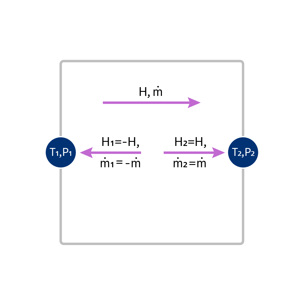
Calculation of energy flow and mass flow from node 1 to node 2 of an approximation model with two nodes.

In the diagram above the following notations are used.

Designations	Description
T₁,P₁	Model node with boundary conditions of temperature temperature_1 and pressure pressure_1
T₂,P₂	Model node with boundary conditions of temperature temperature_2 and pressure pressure_2
N, \(\dot{\mathbf m}\) →	Positive direction of energy flow energy_2 and mass flow rate flowrate_2 of the model

When preparing data for calculating energy flows and mass flow rates within the framework of parametric studies, it is necessary to create:

1. An additional energy flow energy_1 equal to the negative value of energy_2,

2. An additional mass flow rate flowrate_1 equal to negative value of flowrate_2 according to the diagram given above.

2.  Preparing for work

Note

You can download the Jupyter notebook file and the ML model training data if you want to quickly complete this tutorial on your personal computer.

You can also download the ONNX file of the ML model and immediately use it in a project on the REPEAT VISION platform using the Approximation model (P) block.

All subsequent data preparation and ML model creation should be performed on a local machine using the PyTorch framework. It is recommended to run the work in Jupyter.

Before you begin, you need to install:

1. Python package repeat, required for interaction with the REPEAT VISION platform;

2. The repeat_onnx package is used to prepare an additional description of the ML model for its integration into the REPEAT VISION platform via the Approximation model (P) block;

3. Packages for working with data and creating ML models: PyTorch, Scikit-learn, Pandas, ONNX, Matplotlib, tqdm, Jupyter.

In your computer’s command line, you need to run the following commands and continue working in the Jupyter notebook.

Bash

mkdir ml_gas_flow
cd ml_gas_flow
python -m venv repeat_ml.
source repeat_ml/bin/activate
python -m pip install repeat repeat_onnx torch scikit-learn pandas onnx matplotlib tqdm jupyterlab ipywidgets
jupyter lab

PowerShell

mkdir ml_gas_flow
cd ml_gas_flow
python -m venv repeat_ml.
repeat_ml\Scripts\Activate.ps1
python -m pip install repeat repeat_onnx torch scikit-learn pandas onnx matplotlib tqdm jupyterlab ipywidgets
jupyter lab

See also

For more information on using Python on your local machine to interact with the REPEAT VISION platform, please see our tutorials:

1. Using Python in CPython classic implementation

2. Preparing for work on approximating the solution of the differential equation of oscillations using PINN

In the first cell of your notebook, import the Python packages needed to prepare the data and process the calculation results, as well as the Python package repeat with the parametric studies module.

import matplotlib.pyplot as plt
import numpy as np
import onnx
import pandas as pd
import repeat as rp
import repeat.parametric_study as ps
import repeat_onnx as rx
import torch
from pprint import pp
from sklearn.model_selection import train_test_split
from sklearn.preprocessing import StandardScaler
from torch import nn 
from torch import optim
from torch.optim.lr_scheduler import ReduceLROnPlateau
from tqdm.notebook import tqdm

3.  Preparing a model description

In accordance with the required flow ML model, the description of the pneumatic model of machine learning is created in the next cell using the repeat_onnx package to enable subsequent integration of the ML model into the REPEAT VISION platform via the Approximation model (P) block.

Description of the ML model

node_1 = rx.NodeP(
    "Input_unit", "pressure_1", "temperature_1", "flowrate_1", "energy_1"
)
node_2 = rx.NodeP(
    "Output_unit", "pressure_2", "temperature_2","flowrate_2", "energy_2"
)
model_info = rx.ModelP([node_1, node_2])
pp(model_info)

• Lines 1-3. The description of the node #1 of the ML model is created using the NodeP class. The node is assigned the name "Input_unit", which will be displayed in the port properties of the Approximation model (P) block. The arguments are passed the names of the pressure and temperature "pressure_1", "temperature_1" model node, as well as the names of the mass flow rate and energy flow "flowrate_1", "energy_1".

• Lines 4-6. The description of node #2 of the ML model is created using the NodeP class. The second node is assigned the name "Output_unit". The arguments are passed the names of the potentials and flows similar to the first node.

• Line 7. To describe a pneumatic machine learning model, an instance of the ModelP class is created, containing a list of two nodes.

The ML model description model_info will be used in all subsequent stages: data preparation, model creation and its export to the neutral ONNX format.

4.  Data preparation

Note

You can download the Jupyter notebook file if you want to quickly perform the data preparation step on your personal computer.

To subsequently create a machine learning model that approximates the operation of the nozzle, it is necessary to prepare a data set (calculation cases), including:

Input parameters of the ML model

Boundary conditions at the nozzle of the pipeline system:

1. Pressure:

   • "pressure_1"

   • "pressure_2"

2. Temperatures:

   • "temperature_1"

   • "temperature_2"

Output parameters of the ML model

Calculation results for each design case:

1. Mass flow rate of gas:

   • "flowrate_1"

   • "flowrate_2"

2. Energy Flow:

   • "energy_1"

   • "energy_2"

To prepare the required data set, algorithms for performing parametric studies on a model of gas flow in a pipeline system will be required.

Below is a brief description of the main steps for calculating a set of mass flow rates and energy flows on a grid of pressure and temperature parameters of a nozzle model.

First, you need to set up a connection to the REPEAT platform and select a model to perform parametric studies.

user = rp.User(
    "enter a unique API key from REPEAT VISION user cabinet instead of this comment"
)
app = rp.Application(user)
# enter a project ID from REPEAT VISION application instead of 12345
project = 12345
t_interval = rp.TimeInterval(start = 900, end = 1000)
model = app.get_exploration_model(project, t_interval)
print(model, model.existing_variables, sep = "\n")

To prepare the set of input data values, in the next cell, create a dictionary variable_bounds and use the function get_latin_hypercube to create a sparse set of values ​​for the global variables PRESS and TEMP of the pipeline system model.

variable_bounds = dict(
        PRESS = [6.5e6, 9.5e6],
        TEMP  = [10., 30.],
    )
input_data = ps.get_latin_hypercube(
    model, 
    variable_bounds,
    seed = 42,
    sample_size = 800,
    strength = 1,
    optimization = "lloyd"
)
figure, axis = plt.subplots(dpi = 100)
input_data.plot.scatter(x = "TEMP", y = "PRESS", c = "tab:green", marker = ".", ax = axis)
axis.set_xlabel("TEMP $[^{\circ}C]$")
axis.set_ylabel("PRESS $[Pa]$")

As a result of executing the cell code given above, a table of the values ​​of the initial data input_data will be prepared, and a graph of the distribution of a sparse set of values ​​of the pressure and temperature parameters will be displayed.

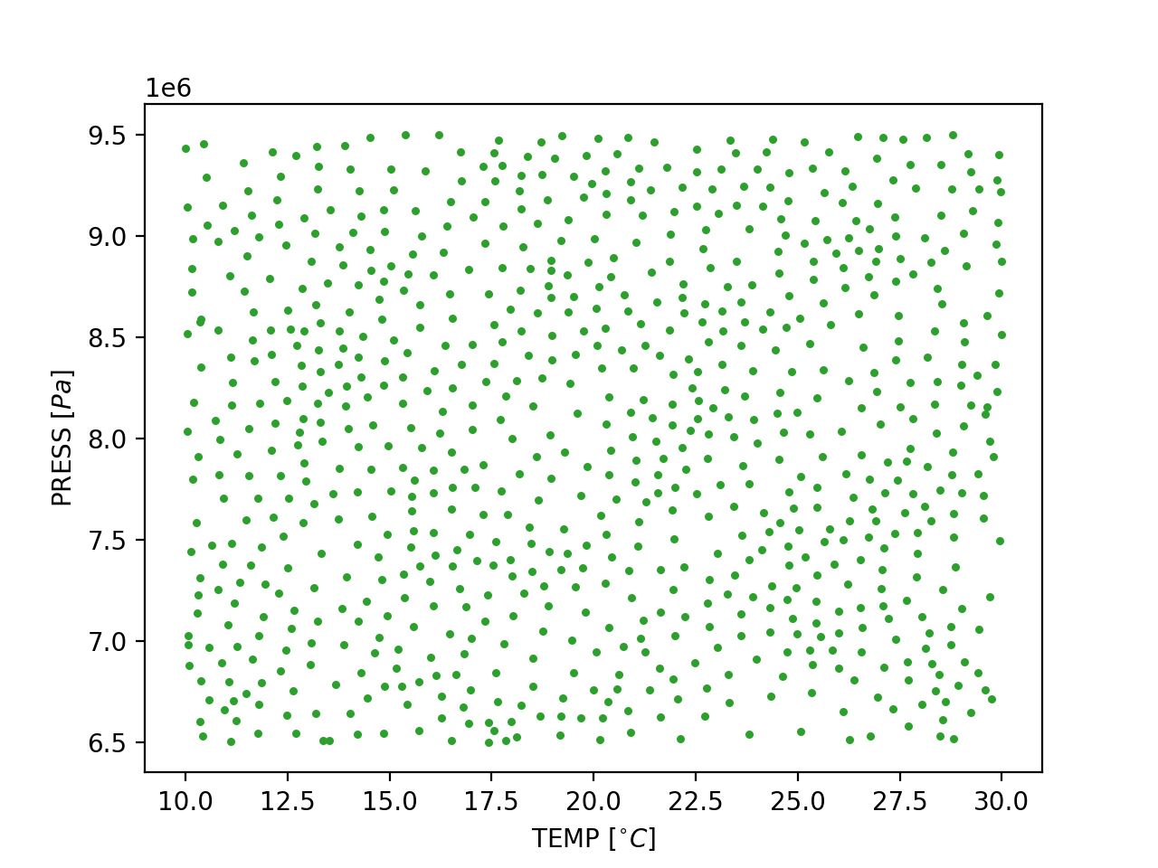
Distribution graph of a sparse set of pressure and temperature parameter values.

See also

A detailed practical guide to performing parametric studies is given in the relevant section of the REPEAT VISION documentation.

The next step is to create a common design_cases table suitable for storing all design cases containing boundary conditions for pressures and temperatures, the names of which are contained in the list model_info.potentials, as well as the values ​​of the results of calculating energy flows and gas mass flow rates for node №2, the names of which are contained in the list node_2.flows.

result_names = [*model_info.potentials, *node_2.flows]
design_cases = input_data.copy(deep = True)
for param in result_names:
    design_cases[param] = pd.NA

design_cases.head()

Next, we need to run a cycle of model calculations on the REPEAT VISION platform. To do this, we create and execute the solve function in the next cell.

def solve(input_data, design_cases):
    for case_num, variables in input_data.iterrows():
        with model as md:
            md.run(variables)
            for param in result_names:
                design_cases.loc[case_num, param] = md.get_results(param).iloc[-1]

solve(input_data, design_cases)

In the next step, the values ​​of mass flow rate "flowrate_1" and energy flow "energy_1" are calculated in accordance with the requirements for the machine learning model for further integration into the REPEAT VISION platform.

design_cases[node_1.flows] = - design_cases[node_2.flows]

Hint

In the process of calculating the values ​​of mass flow rate "flowrate_1" and energy flow "energy_1" in the cell above, the object node_1 is used, which stores the names of the calculated values ​​in the flows attribute, formed earlier when describing node №1 of the ML model.

Next, you need to save the table of design cases design_cases in case you create other ML models using the already obtained modeling results.

design_cases.to_csv("gas_flow_data.csv")

5.  Analysis of calculation results

To display the calculation results, it is necessary to create an auxiliary function for three-dimensional visualization based on the capabilities of the matplotlib package.

def plot_3d_scatter(table, column = "flowrate_2", units = "$[kg/s]$", c = "tab:blue"):
    fig = plt.figure(dpi = 200)
    ax = fig.add_subplot(projection = "3d")
    ax.scatter(
        table["pressure_2"], 
        table["temperature_2"], 
        table[column], 
        marker = ".",
        c = c
      )
    ax.view_init(azim = 240)
    ax.set_xlabel("pressure_2 $[Pa]$")
    ax.set_ylabel("temperature_2 $[^{\circ}C]$")
    ax.set_zlabel(f"{column} {units}")
    fig.savefig(f"results_{column}.png")
    plt.show()

Next, it is necessary to call an auxiliary function to display the three-dimensional dependence of the selected flow on potentials. First, the function plot_3d_scatter is passed only the table of design cases design_cases to display the mass flow rate flowrate_2 as a function of the pressure pressure_2 and the temperature temperature_2 at the nozzle outlet.

plot_3d_scatter(design_cases)

The graph shows the dependence of the mass flow rate on the pressure and temperature at the outlet of the nozzle (block №14 Orifice (P), node №2 ML model).

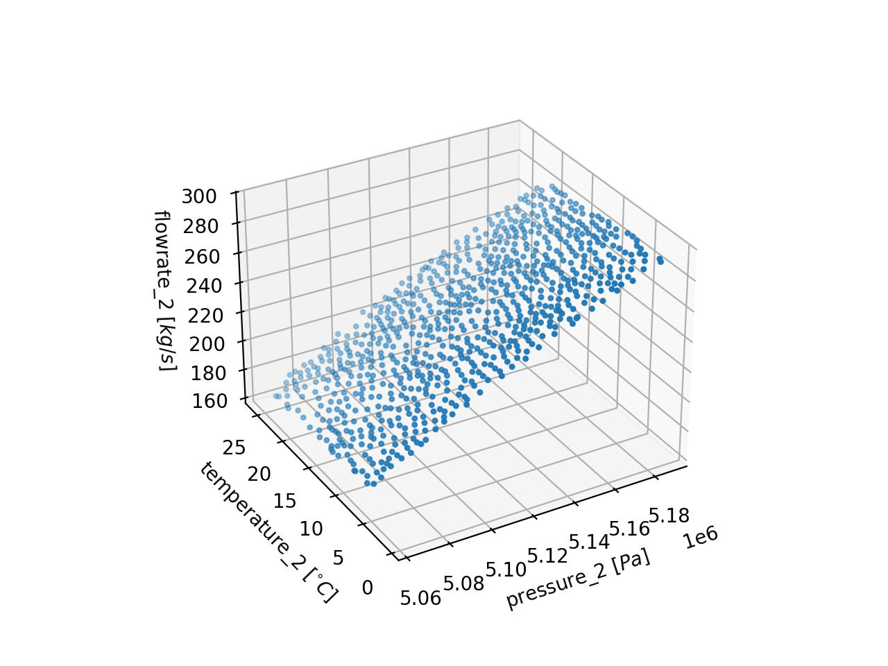
Results of calculation of mass flow depending on pressure and temperature at the outlet of the nozzle

In the next step, the helper function plot_3d_scatter is called to display the energy flux energy_2.

plot_3d_scatter(design_cases, "energy_2", "$[W]$", "tab:orange")

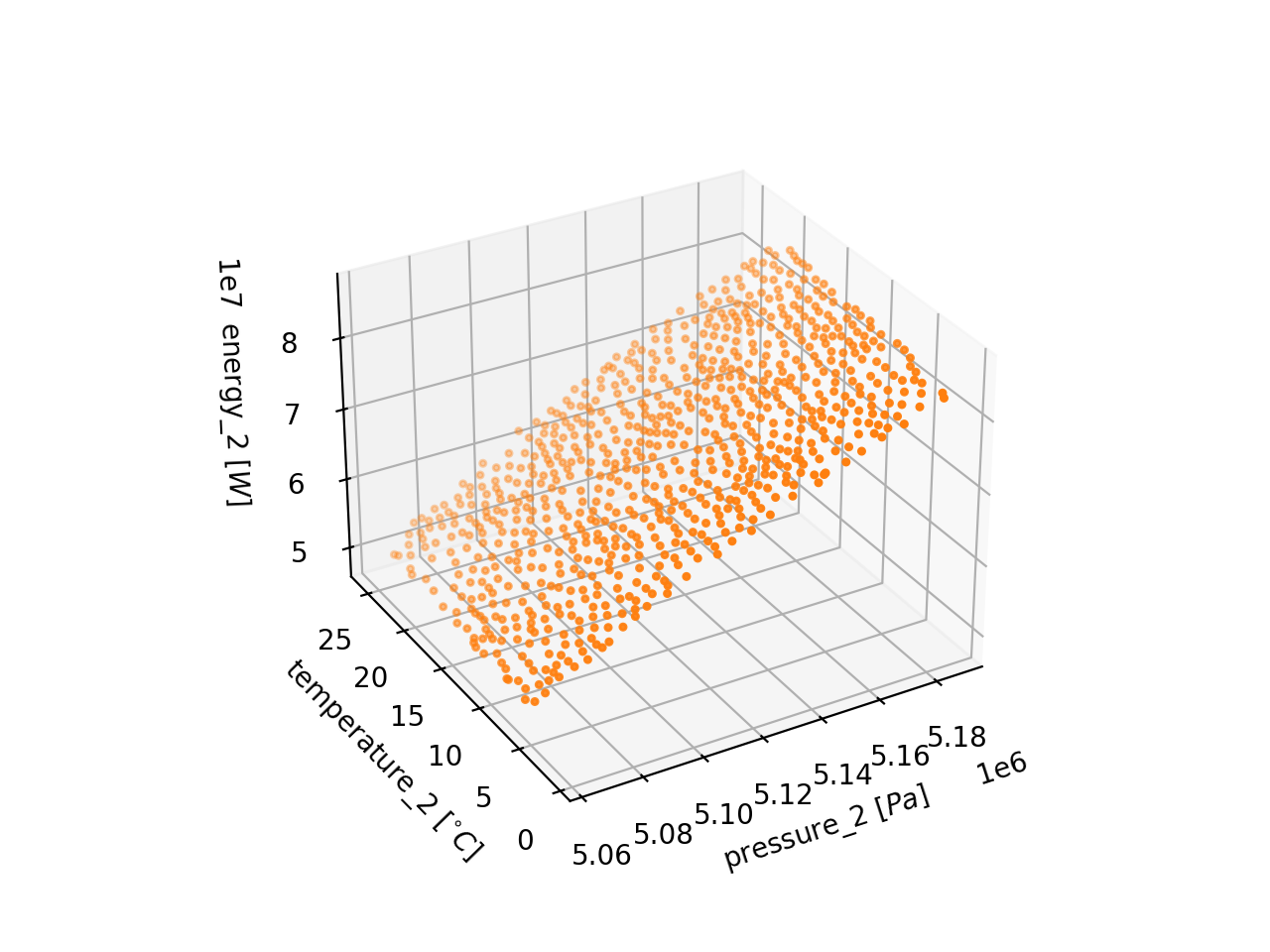
Results of calculating the energy flow depending on the pressure and temperature at the outlet of the nozzle

In the graphs shown above, it is necessary to note the difference in the orders of magnitude of the model parameters (see table below).

Model parameter	Order
Gas mass flow	2
Flow of energy	7
Temperature	1
Pressure	6

Conclusions based on the results of graph analysis

1. Gas mass flow rate, energy flow and temperature have a non-linear dependence on pressure;

2. The model parameters have significantly different orders of magnitude.

The findings directly impact the choice of machine learning model architecture that will be developed in the next section.

6.  Data preprocessing

In this section, we will perform the steps of preparing the calculated data for the process of training and testing the ML model.

First, you need to create a dictionary dict to store the following settings.

Key	Setting Description
"device"	The device that will be used to train the model on your local machine
"dtype"	The data type used in the torch.tensor tensors of the PyTorch framework in accordance with the [general requirements](../../../reference/blocklib/externalModels/ApproximationOnnx/index.md #ml-model-common-requirements) for ML models

TENSOR_SETTINGS = {
    "device" : "cuda" if torch.cuda.is_available() else "cpu",
    "dtype" :  torch.double,
}

In the next cell, you need to prepare some helper functions.

def to_tensor(data) -> torch.tensor:
    return torch.tensor(data, **TENSOR_SETTINGS)

def to_column_tensor(data):
    return to_tensor(data).reshape(-1, 1)

Next, we need to create a helper function get_torch_tensors to prepare torch.tensor data structures from a set of pandas.DataFrame tables.

def get_torch_tensors(tables : list[pd.DataFrame]):
    total = []
    for table in tables:
        tensors = {}
        for key, values in table.items():
            tensors[key] = to_column_tensor(values.to_numpy())
        
        total.append(tensors)
    
    return total

In the next cell, using the train_test_split function of the scikit-learn library, the previously prepared data is split into a training set and a testing set.

potential_train, potential_test, flow_train, flow_test = train_test_split(
  design_cases[model_info.potentials], design_cases[model_info.flows], 
  test_size = 0.33, random_state = 42
)

Line 2 of the code cell above uses the following lists to easily separate the data:

1. List of potentials model_info.potentials - pressures and temperatures in model nodes, ['pressure_1', 'temperature_1', 'pressure_2', 'temperature_2'];

2. List of flows model_info.flows - ​​mass flow rates and energy flows in model nodes, ['flowrate_1', 'energy_1', 'flowrate_2', 'energy_2'].

These lists were configured earlier during preparing the ML model description.

In the next step, using the previously created get_torch_tensors function, the torch.tensor data structures of the model potentials are prepared for subsequent training and testing of the ML model.

potential_train_tensor, potential_test_tensor = get_torch_tensors(
  (potential_train, potential_test)
  )

6.1.  Data standardization

Now it is necessary to perform a step based on the results of the previously performed data analysis, which revealed a significant difference in the orders of magnitude of the model parameters.

An instance of the StandardScaler class of the scikit-learn library is created on the training sample of model potentials for subsequent calculation of the average value of the potentials and their standard deviation.

potential_scaler = StandardScaler()
potential_scaler.fit(potential_train)

Important

Standardization allows to linearly transform the data to zero mean and unit SD in order to further ensure the convergence of the optimizer solution while minimizing the residual calculated by the loss function during the training of the ML model.

The next step is to standardize the model flows.

flow_scaler = StandardScaler()
flow_scaler.fit(flow_train)
flow_train_scaled = to_tensor(flow_scaler.transform(flow_train))
flow_test_scaled = to_tensor(flow_scaler.transform(flow_test))

Lines 3 and 4 of the code cell above standardize the training and testing samples of the model streams and convert them into torch.tensor data structures using the previously created to_tensor function.

Next, it is necessary to prepare the mean values and SD of the potentials and flows of the model.

summary = dict(
    potential_mean = to_tensor(potential_scaler.mean_),
    potential_scale = to_tensor(potential_scaler.scale_),
    flow_mean = to_tensor(flow_scaler.mean_),
    flow_scale = to_tensor(flow_scaler.scale_),
)

The SD and average values ​​of the model parameters calculated above will be used further in describing the architecture of the machine learning model.

7.  Creating a machine learning model of gas flow through a nozzle

The next step is to create a machine learning model using the PyTorch framework. To approximate the process of gas flow through a nozzle, it is necessary to create a model of a multilayer neural network, which is chosen due to the nonlinearity of the flow dependencies on the potentials identified as a result of the analysis of the obtained data.

7.1.  Creating an initialization method

The description of the ML model must begin with the initialization method of the ModelOrifice class, which inherits the base class nn.Module neural network of the PyTorch framework.

Description of the initialization of the ML model of gas flow through a nozzle

class ModelOrifice(nn.Module):
    def __init__(self, potential_mean, potential_scale, flow_mean, flow_scale,
                 hidden_size = 128):
        super().__init__()
        self.common_part = nn.Sequential(
            nn.Linear(4, hidden_size),
            nn.LayerNorm(hidden_size),
            nn.Tanh(),
            nn.Linear(hidden_size, hidden_size),
            nn.LayerNorm(hidden_size),
            nn.Tanh()
        )
        self.flowrate_part = nn.Linear(hidden_size, 1, bias = False)
        self.energy_part = nn.Linear(hidden_size, 1, bias = False)
        self.potential_mean = potential_mean
        self.potential_scale = potential_scale
        self.flow_mean = flow_mean
        self.flow_scale = flow_scale

• Lines 2-3. To initialize an instance of the neural network ModelOrifice class, it is necessary to pass the previously created mean values ​​and SD of the model potentials and flows as arguments.

• Line 5. In the ML model’s common_part attribute, a sequence of two layers of neurons is created using the nn.Sequential class. The sequence is intended to perform general transformations of the model’s input parameter data.

• Line 6. In the common ML model component common_part, the first class created is a linear transformation class nn.Linear, which takes four parameters (pressures and temperatures at two model nodes) and calculates an intermediate result for the neurons of the next layer, the number of which is configured using the hidden_size argument.

• Lines 7-8. Next, in the common_part component, the nn.LayerNorm class is created to perform normalization of the parameter values ​​in the first layer of neurons. Also, the nn.Tanh class is created to activate the neurons of the next layer according to the hyperbolic tangent function.

• Lines 9-11. In the common_part component, a second layer of neurons is created, similar to the first layer.

• Lines 13-14. Separate nn.Linear ML model components are created, the coefficients of which are adjusted separately for approximating the gas mass flow rate in the flowrate_part method, and for calculating the gas energy flux in the energy_part method. The flowrate_part and energy_part methods account for significant differences in orders of magnitude between gas mass flow data and energy flow data.

• Lines 15-18. The attributes of the mean values ​​and SD of the potentials and flows of the model are created.

7.2.  Creating the forward method

At this stage, the forward method is created, which determines the order in which input data passes through the network.

Description of the forward method of the ModelOrifice class

    def forward(self, pressure_1, temperature_1, pressure_2, temperature_2):
        x = torch.cat([pressure_1, temperature_1, pressure_2, temperature_2], 
                      dim = 1)
        x_scaled = (x - self.potential_mean) / self.potential_scale
        common_results = self.common_part(x_scaled)
        flowrate_2 = self.flowrate_part(common_results)
        energy_2 = self.energy_part(common_results)
        flowrate_1 = - flowrate_2
        energy_1 = - energy_2
        flows = torch.cat([flowrate_1, energy_1, flowrate_2, energy_2], 
                          dim = 1)
        if self.training: 
            return flows
        
        return self.postprocessing(flows)

• Line 20. The forward method of the ModelOrifice class is created, whose input arguments are torch.tensor structures containing pressure and temperature data for two model nodes.

• Lines 21-22. The initial parameters are prepared. The pressures and temperatures of two model nodes are combined into a common tensor for transfer to the first layer of the model. The parameters are combined column-wise (dim = 1).

• Line 23. Standardization of ML model potentials is performed to eliminate differences in the orders of magnitude of model potential values.

• Line 24. Intermediate calculation of flows in the common component common_part of the ML model is performed.

• Lines 25-26. The gas mass flow rate and energy flow are calculated in the flowrate_part and energy_part methods, respectively, for node №2 of the ML model.

• Lines 27-28. The flows for node №1 of the ML model are calculated in accordance with the previously completed problem formulation.

• Lines 29-30. Streams are prepared for two model nodes. The parameters are merged by columns dim = 1. The streams are combined into a common tensor for subsequent transfer to the loss function or to the function for processing the calculation results depending on the state of the model: the training state or the calculation state.

• Lines 31-34. When the model is trained, self.training is set to True and the estimated flow values ​​are passed to the loss function. Otherwise, the results of the model flow calculations are processed (this process is described in the next section).

7.3.  Creating a method for processing calculation results

At the final stage of describing the neural network class, it is necessary to describe the methods for processing the results of calculating the mass flow rate of gas and energy flow for two model nodes. Processing the results of flow calculations is necessary during the direct operation of the ML model (Machine learning Inference) after completing the ML model training process.

During the processing of calculation results, the standardized values ​​of the model flows are converted to the original scale of the gas mass flow rate and energy flow.

Description of methods for processing flow calculation results

    def postprocessing(self, flows):
        orig_flows = flows * self.flow_scale + self.flow_mean
        columns = range(flows.shape[1])
        
        return [self.get_column_vector(orig_flows, i) for i in columns]

    def get_column_vector(self, tensor, column):
        return tensor[:, column].reshape(-1, 1)

• Line 36. The postprocessing method of the ModelOrifice class is created, taking as an argument the flows tensor containing the gas mass flow rates and energy flows for two model nodes.

• Line 37. Gas mass flow rates and energy flows are converted to the original scale.

• Line 40. In accordance with the data structure requirements of the neutral ONNX format and the REPEAT VISION platform, the flux tensor is converted by the get_column_vector method into a list of column vectors for each model node, which must contain the mass flow rate and energy flow of the gas.

7.4.  All model code

For ease of use, the entire code for a multilayer neural network class, designed to approximate the process of gas flow through a nozzle, is provided below.

Description of the ModelOrifice class

class ModelOrifice(nn.Module):
    def __init__(self, potential_mean, potential_scale, flow_mean, flow_scale,
                 hidden_size = 128):
        super().__init__()
        self.common_part = nn.Sequential(
            nn.Linear(4, hidden_size),
            nn.LayerNorm(hidden_size),
            nn.Tanh(),
            nn.Linear(hidden_size, hidden_size),
            nn.LayerNorm(hidden_size),
            nn.Tanh()
        )
        self.flowrate_part = nn.Linear(hidden_size, 1, bias = False)
        self.energy_part = nn.Linear(hidden_size, 1, bias = False)
        self.potential_mean = potential_mean
        self.potential_scale = potential_scale
        self.flow_mean = flow_mean
        self.flow_scale = flow_scale
    
    def forward(self, pressure_1, temperature_1, pressure_2, temperature_2):
        x = torch.cat([pressure_1, temperature_1, pressure_2, temperature_2], 
                      dim = 1)
        x_scaled = (x - self.potential_mean) / self.potential_scale
        common_results = self.common_part(x_scaled)
        flowrate_2 = self.flowrate_part(common_results)
        energy_2 = self.energy_part(common_results)
        flowrate_1 = - flowrate_2
        energy_1 = - energy_2
        flows = torch.cat([flowrate_1, energy_1, flowrate_2, energy_2], 
                          dim = 1)
        if self.training: 
            return flows
        
        return self.postprocessing(flows)
    
    def postprocessing(self, flows):
        orig_flows = flows * self.flow_scale + self.flow_mean
        columns = range(flows.shape[1])
        
        return [self.get_column_vector(orig_flows, i) for i in columns]

    def get_column_vector(self, tensor, column):
        return tensor[:, column].reshape(-1, 1)

7.5.  Description of the ML model training process

After creating the ModelOrifice class, which describes the neural network model, it is necessary to configure the optimizer, which is designed to determine the unknown weights of the ML model in the process of minimizing the loss function.

Description of the optimizer settings for training an ML model

torch.manual_seed(42)
model = ModelOrifice(hidden_size = 180, **summary).double().to(TENSOR_SETTINGS["device"])
criterion = nn.MSELoss()
optimizer = optim.AdamW(model.parameters(), lr = 1e-3, weight_decay = 1e-3)
scheduler = ReduceLROnPlateau(optimizer, "min", factor = 0.5, patience = 50) 
num_epochs = 3000
train_losses, test_losses = [], []

• Line 2. Initialization of an instance of the ModelOrifice model class, switching the model to double-precision mode using the .double() method in accordance with the requirements of the REPEAT VISION platform for ML models. Additionally, the ML model is passed the settings about the device used TENSOR_SETTINGS["device"] to perform the machine learning process.

• Line 3. Initialization of the loss function criterion, which uses the mean squared error as a criterion for the quality of the ML model.

• Line 4. Initialization of the AdamW optimizer. The values ​​of the lr = 1e-3 (learning rate) and weight_decay = 1e-3 settings are determined empirically.

• Строка 5. Инициализация экземпляра класса планировщика ReduceLROnPlateau. Планировщик предназначен для уменьшения значения скорости обучения (learning rate), когда прекращается уменьшение среднеквадратичной ошибки.

• Lines 6-7. The variable num_epochs = 3000 is created, which defines the number of epochs for training the ML model. Lists are also created to store the values ​​of the loss function for the training and testing data sets for the purpose of further analysis of the convergence process of the ML model quality criterion value.

After setting up the optimizer, the ML model training cycle is described next.

Description of the model training cycle

for epoch in range(num_epochs):
    model.train()
    optimizer.zero_grad()
    outputs_train = model(**potential_train_tensor)
    loss_train = criterion(outputs_train, flow_train_scaled)
    loss_train.backward()
    optimizer.step()
    model.eval()
    with torch.no_grad():
        model.train() 
        outputs_test = model(**potential_test_tensor)
        model.eval()
        loss_test = criterion(outputs_test, flow_test_scaled)
    
    scheduler.step(loss_test)
    train_losses.append(loss_train.item())
    test_losses.append(loss_test.item())

• Lines 2-7. The typical part of determining the ML model weights on the training data set is performed, a detailed description of which is given in the tutorial Approximation of the solution of the differential equation of oscillations using PINN.

• Lines 8-15. In the model evaluation mode, the residual is calculated on the test dataset potential_test_tensor for subsequent transmission of the loss_test values ​​to the scheduler scheduler.

• Lines 16-17. Saving the values ​​of the ML model quality criteria calculated on the training and testing data sets is performed.

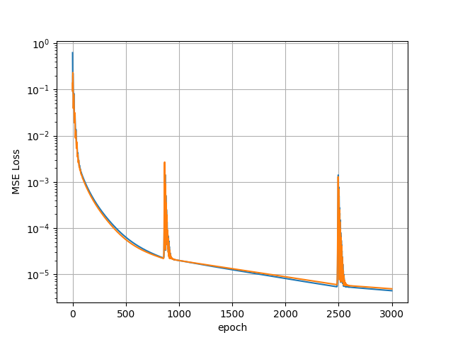
Mean squared error values ​​depending on the model training epoch for the training and validation datasets

The following notations are used in the graphs above.

Lines	Description
Blue Line	Dependence of the root mean square error on the iteration number on the training data set
Orange Line	Dependence of the root mean square error on the iteration number on the validation data set

7.6.  Saving an ML model to an ONNX file

At the end of the ML model creation process, the machine learning model is saved in the neutral ONNX format used by the REPEAT VISION platform for integration of approximation models for use in structural modeling.

Description of the settings for saving a model to ONNX format

onnx_file = "model_orifice.onnx"
model.eval()
torch.onnx.export(
    model,
    args = (to_column_tensor(6456249.5),
            to_column_tensor(19.912780),
            to_column_tensor(5065394.0),
            to_column_tensor(16.410051),
            ),
    f = onnx_file,
    opset_version = 17,
    input_names = model_info.potentials,
    output_names = model_info.flows,
    )

• Line 1. The string variable onnx_file is created, containing the name of the ONNX file to be saved to, where the machine learning model will be written.

• Line 2. The ML model is switched to calculation mode to calculate the parameters of gas mass flow rate and energy flow at the original scale.

• Line 4. The torch.onnx.export() function’s first argument is the previously trained model model.

• Lines 5-9. The named argument args is passed the values ​​of the default pressure and temperature boundary conditions. The data structure used is a 1x1 torch.tensor with the torch.double type, in accordance with the requirements of the REPEAT VISION platform for the ML model. The default values ​​are one of the test cases from the previously obtained dataset.

• Lines 10. The named argument f is passed the name of the ONNX file to be saved from the previously created onnx_file variable for subsequent use on the REPEAT VISION platform.

• Lines 12. The named argument input_names is assigned a list of names of pressure and temperature boundary conditions. The potentials list from the model_info object of the previously prepared description ML model is used.

• Lines 13. The named argument output_names is passed a list of names of the mass flow and energy flow calculation results for two ML model nodes. The flows list from the model_info object of the previously prepared description is used.

Next, the necessary information about the ML model is written into a neutral ONNX file in accordance with the REPEAT VISION platform requirements for an additional model description.

Writing an additional description of the ML model to an ONNX file

properties = onnx.StringStringEntryProto()
properties.key = "repeat_contract"
properties.value = model_info.to_onnx()
model_onnx = onnx.load(onnx_file)
model_onnx.metadata_props.append(properties)
onnx.save(model_onnx, onnx_file)

• Line 1. The properties data structure is created using the onnx package.

• Line 2. The key attribute is passed the string value of the "repeat_contract" key, by which the Approximation model (P) block will search for the necessary settings.

• Line 3. The value attribute is passed the previously prepared additional description of the ML model by calling the to_onnx() method of the model_info object. The description of the model will allow the block Approximation model (P) to ensure the transfer of pressures and temperatures to the nodes of the ML model, and as a result of the calculation to obtain the mass flow and energy flow.

• Lines 4-6. The ONNX file with the previously saved ML model is read and the properties object is added to the metadata_props structure. Finally, the ONNX file is overwritten with the ML model, properties. Finally, the ONNX file is overwritten with the ML model, containing an additional description.

8.  Integration of the ML model into the REPEAT VISION platform

To complete the work, you need to load the ML file of the model_orifice.onnx model into the REPEAT VISION platform using the Approximation model (P) block into the previously used project.

It is necessary to copy and paste the previously created blocks Reservoir (P) №2 and №5, as well as Pipe (P) №1 and №3. It is also necessary to add the Flow Rate Sensor (P) №29 block, which should output the mass flow rate \([kg/s]\) measured in the Pipe (P) №25, to the Outport №30 block.

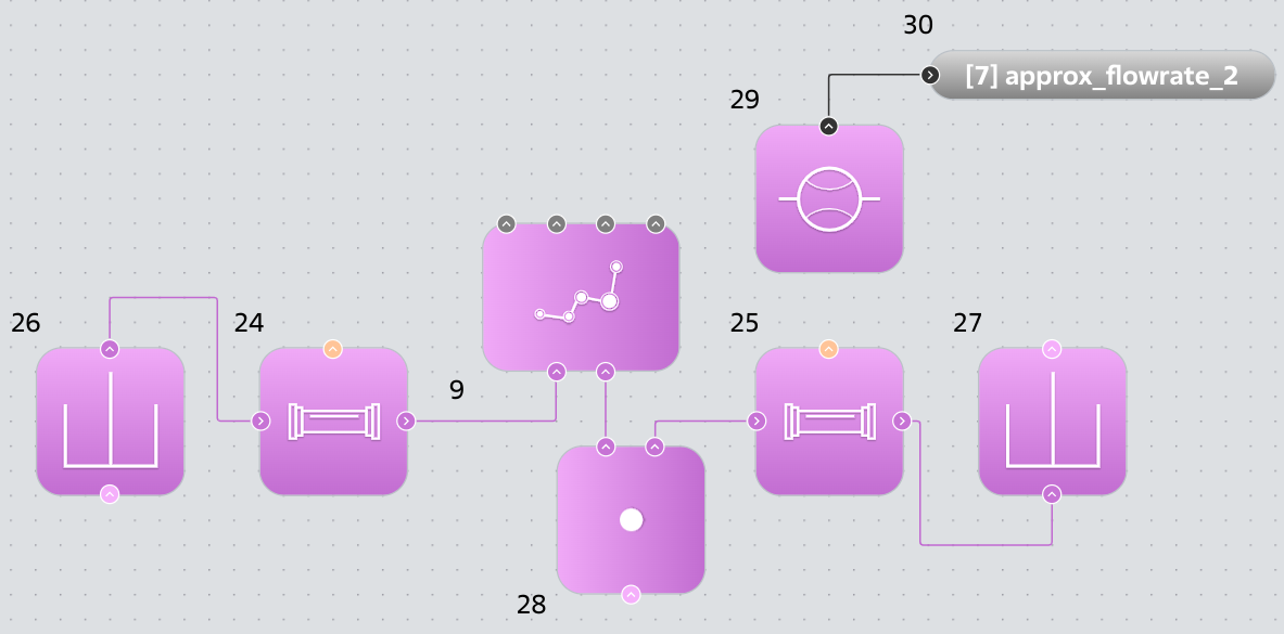
A pipeline system with a block approximating the process of gas flow through a nozzle.

The entire project, containing a pipeline system for simulating gas flow through a nozzle, as well as a system with a block Approximation model (P), is shown in the diagram given below.

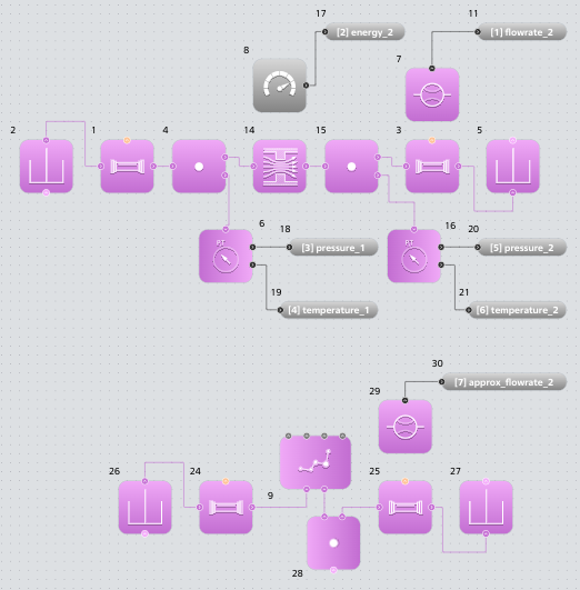
Pipeline systems design

It is necessary to save this project with a new name and perform independent testing of the ML model approximating the process of gas flow through the nozzle.

9.  Testing a machine learning model

Note

You can download the Jupyter notebook file if you want to quickly run the testing step of a machine learning model.

To independently quantitatively evaluate the quality of the ML model, the approximation model is tested on the REPEAT VISION platform using reference results of calculating the mass flow rate of gas in a pipeline system created previously.

The testing process is proposed to be performed using Python, using the previously created parametric study script. Copying and modifying it results in the test program presented below.

In the first cell, you need to perform standard actions to import the required modules, and you also need to create objects for interaction with the REPEAT VISION platform.

import matplotlib.pyplot as plt
import numpy as np
import pandas as pd
import repeat as rp
import repeat.parametric_study as ps


user = rp.User(
    "enter a unique API key from REPEAT VISION user cabinet instead of this comment"
)
app = rp.Application(user)
# enter a project ID from REPEAT VISION application instead of 12345
project = 12345
app = rp.Application(user)
t_interval = rp.TimeInterval(start = 900, end = 1000)
model = app.get_exploration_model(project, t_interval)
print(model, model.existing_variables, sep = "\n")

Next, you need to create a set of values ​​for the pressure and temperature parameters using the get_cartesian_product function.

variable_values = dict(
    PRESS = np.linspace(6.75e6, 9.42e6, num = 21),
    TEMP = np.array([20.]),
)
input_data = ps.get_cartesian_product(model, variable_values)

It is also necessary to create a common table design_cases, suitable for storing all design cases containing boundary conditions for temperatures and pressures, as well as the values ​​of the mass flow calculation results:

1. "flowrate_2" - reference values ​​of mass flow in the pipeline system for simulating gas flow through a nozzle;

2. "approx_flowrate_2" - mass flow rate values ​​obtained in the pipeline system with a block approximating the process of gas flow through a nozzle.

result_names = ["flowrate_2", "approx_flowrate_2"]
design_cases = input_data.copy(deep = True)
for param in result_names:
    design_cases[param] = pd.NA

design_cases.head()

The next step is to create and execute the solve function that was used earlier in the parametric studies.

def solve(input_data, design_cases):
    for case_num, variables in input_data.iterrows():
        with model as md:
            md.run(variables)
            for param in result_names:
                design_cases.loc[case_num, param] = md.get_results(param).iloc[-1]

solve(input_data, design_cases)

Next, based on the obtained results of independent calculations, the relative deviation of the approximated values ​​flow_approx from the reference values ​​of the mass flow flow_exact is calculated using the calc_relative_error function.

def calc_relative_error(flow_exact, flow_approx):
    return (flow_exact - flow_approx).abs() / flow_exact * 100

design_cases["error"] = calc_relative_error(
    flow_exact = design_cases["flowrate_2"], 
    flow_approx = design_cases["approx_flowrate_2"]
    )

In the next step, a plot is created to compare the ML model calculation results with the reference mass flow rate results.

ax = design_cases.plot(x = "PRESS", y = "flowrate_2", c = "tab:blue")
design_cases.plot.scatter(x = "PRESS", y = "approx_flowrate_2", c = "tab:red", ax = ax)
ax.set_xlabel("pressure $[Pa]$")
ax.set_ylabel("flowrate $[kg/s]$")

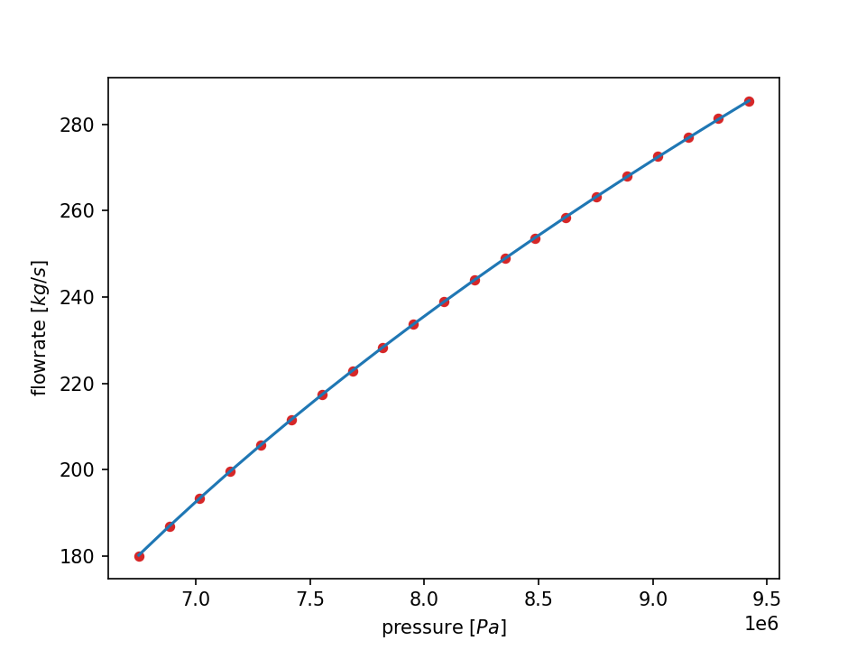
Graph of mass flow rate versus pressure in a tank.

The following notations are used in the graph above.

Lines	Description
Blue Line	Dependence of mass flow rate on pressure in a pipeline system tank for modeling gas flow through a nozzle
Red Dots	Dependence of approximated mass flow values ​​on tank pressure of a pipeline system with an integrated machine learning model

print(f'{design_cases["error"].max() :.3f} %')

The maximum relative deviation of the approximated values ​​from the reference mass flow values ​​is 0.095%. This result demonstrates the applicability of neural network algorithms for approximating gas flow models in system simulation on the REPEAT VISION platform.

10.  Conclusions

As a result of completing this practical guide:

1. You have become familiar with the process of preparing a machine learning model to approximate the process of gas flow through a nozzle using the REPEAT VISION platform and PyTorch;

2. You have learned how to integrate a model into the REPEAT VISION ML platform using the Approximation model (P) block to solve problems of modeling gas flow in pipeline systems;

3. You have become familiar with the capabilities of the Python package repeat_onnx which provided the integration of the ML model into the REPEAT VISION platform, simplified the process of data preparation and the process of creating the ML model;

4. You have become familiar with testing a machine learning model both during its creation and during its operation on the REPEAT VISION platform.