Modeling of zero-sequence current directional protection of 220 kV power transmission lines

 Continuing the theme of device modeling RP&A (see the practical guide Differential current protection of power transformer), this practical guide provides an overview of the zero-sequence directional overcurrent protection (ZDOP) model for a power transmission line (PTL) and reproduces its operation within a two-machine power system model. The considered ZDOP model is available in the Demo Projects section.

Note

When reviewing this practical guide, we recommend familiarizing yourself with the demo project [DEMO] 220 kv transmission line zero sequence directional overcurrent protection.

 This practical guide will cover:

• the operating logic of the ZDOP PTL based on the ШЭ2607 016 cabinet by «EKRA» and its implementation in REPEAT VISION;

• constructing vector diagrams for the zero-sequence power directional relay (ZPDR) using the REPEAT VISION - embedded JupyterLite notebook;

• The operation of the developed ZDOP model under various disturbances in the test power system scheme.

1.  ZDOP model

1.1.  Description of the power system model

 Fig. 1 shows the structural diagram of a two-machine power system with ZDOP for a transmission line.

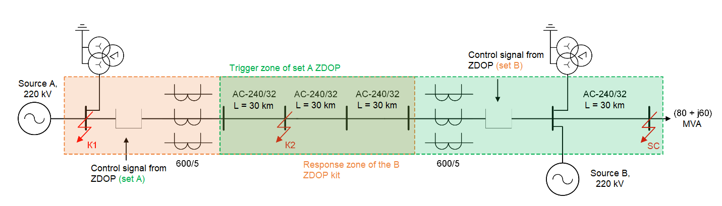
Fig. 1 Structural diagram of the power system for studying ZDOP PTL operation

 The power system in Fig. 1 contains:

• two voltage sources of 220 [kV];

• two PTL with lengths of 90 [km] and 30 [km];

• a load with a power of (80 + j60) [MVA];

• power circuit breakers;

• measuring current transformers (CT) and voltage transformers (VT).

 The protected object is a 220 [kV] PTL with a total length of 90 [km] (for simulating SC, the line is divided into 3 sections of 30 [km] each). The protected PTL is equipped with 2 protection sets:

• set A from the side of source A;

• set B from the side of source B.

Note

Fig. 1 also shows the operating zones for each protection set, considering the directional nature of the protections into the line.

 The parameters of the scheme elements are given in tables 1 - 2.

Table 1 Parameters for modeling the power source [1], (Table 3.8)

Source	\(U_{nom}\) [kV]	Connection line length, [km]	Conductor brand	Catalog data \(r_0\), [Ohm/km]	Catalog data \(x_0\), [Ohm/km]	Calculated parameters \(l_0\), [H/km]	Calculated parameters R, [Ohm]	Calculated parameters L, [H]
Source A	220\(\cdot\)0.9	20	АС-240/32	0.118	0.435	0.001385	2.36	0.0277
Source B	220\(\cdot\)0.9	100	АС-240/32	0.118	0.435	0.001385	11.8	0.1385

Table 2 Parameters for modeling the PTL [1], (Table 3.8)

Length, [km]	Conductor brand	Catalog data \(r_0\), [Ohm/km]	Catalog data \(x_0\), [Ohm/km]	Catalog Data \(b_0\), [S/km]	Calculated parameters \(l_0\), [H/km]	Calculated Parameters \(c_0\), [F/km]
90	АС-240/32	0.118	0.435	2.604\(\cdot10^{-6}\)	0.001385	8.289\(\cdot10^{-9}\)
30	АС-240/32	0.118	0.435	2.604\(\cdot10^{-6}\)	0.001375	8.289\(\cdot10^{-9}\)

1.2.  Description of the ZDOP model

 Zero-sequence current directional protection is used as backup protection against earth SCs as part of the protection set for PTLs with voltages of 110 [kV] and above. ZDOP is a protection with relative selectivity (i.e., it responds to faults both within the protected line zone and in the adjacent line/transformer zone) and includes several stages with different coverage of the protected line and stepped time delay characteristics [2].

 The operating logic of the ZDOP is implemented based on the ШЭ2607 016 line protection cabinet by “EKRA” [3]. A simplified functional diagram of the logical part of the ZDOP [4] is shown in Fig. 2.

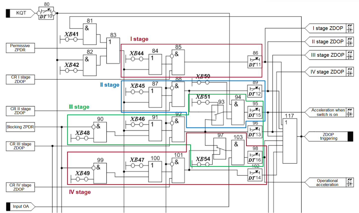
Fig. 2 Simplified functional diagram of the logical part of ZDOP ШЭ2607 016

 The studied protection is four-stage, all stages have directionality (i.e., they operate based on a specific direction of zero-sequence power, determined by the ZPDR). The directionality of stages I and II is ensured by the operation of the permissive power relay (elements 84 and 87), and the directionality of stages III and IV is ensured by the operation of the permissive or non-operation of the blocking power relay (elements 91 and 100).

Note

The blocking relay is used when the sensitivity of the permissive ZPDR might be insufficient (e.g., on long PTL connected to powerful sources, with small zero-sequence impedances of the system adjacent to the protection installation site) [2]. It is worth noting that in the considered ZDOP model, the use of the blocking relay is not related to the sensitivity of the permissive ZPDR.

 The operating logic of the circuit in Fig. 2 is as follows: the value of the triple zero-sequence current \(3I_0\) is compared with the \(3I_0\) current setting of each stage. If the setting for any stage is exceeded, the current relay (CR) operates. If the required directionality of the zero-sequence power is also provided (a logical ‘1’ appears at the outputs of elements 84, 87, 91, 100), then a trip signal for the circuit breaker is generated (elements 85, 88, 92, 101) with a specified time delay (elements 86, 89, 96, 102).

Note

Fig. 2 also shows elements for generating a trip signal during operational acceleration (elements 97, 103, 98) and protection acceleration upon breaker closing (elements 93, 94, 95). In the considered ZDOP model, these functions are not implemented, but you can add them yourself if necessary.

 The ZDOP model discussed further is implemented in REPEAT VISION using the Jython block, blocks from the Automation and Electronics libraries. The latter are used to model the current circuits in the protection terminal.

1.3.  Formation of Triple zero-sequence current and voltage

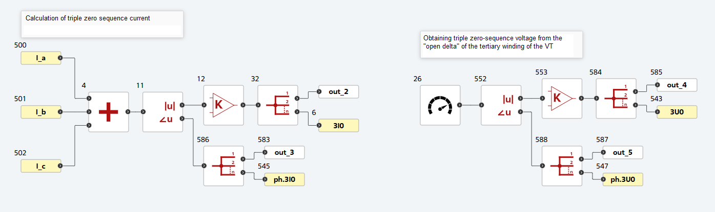
Fig. 3 Formation of 3I0 and 3U0 in the ZDOP scheme

 Fig. 3 shows a fragment of the ZDOP scheme where the RMS value and phase of the triple zero-sequence current and voltage are obtained using the Fourier blocks №11 and №552 and the Gain (blocks №12 and №553 with a gain of 1/√2). The value \(3I_0\) is calculated from the phase currents using formula (1):

(1)\[3 \dot I_0= \dot I_{А-НН}+ \dot I_{В-НН}+ \dot I_{С-НН}\]

where \( \dot I_{А-НН}, \dot I_{В-НН}, \dot I_{С-НН}\) are the vectors of the phase currents from the secondary windings of the CT.

The value \(3U_0\) is formed by connecting the tertiary winding of the VT in an “open delta” configuration (see item 2).

1.4.  Implementation of the operating logic for the permissive and blocking zero-sequence power directional relays

 Fig. 4 shows a fragment of the ZDOP scheme with the operating logic of the permissive ZPDR. Fig. 5 shows vector diagrams explaining the operation of the ZPDR.

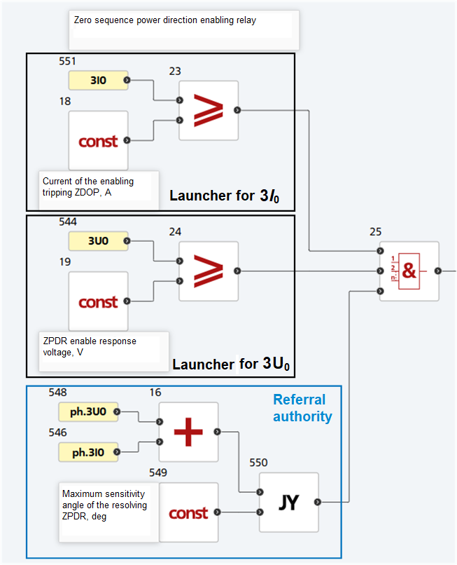
Fig. 4 Implementation of the permissive ZPDR logic in the ZDOP scheme

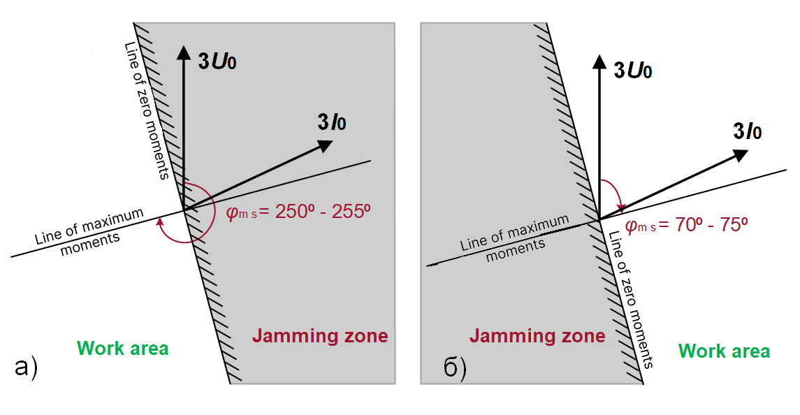
Fig. 5 Vector diagrams of the permissive (a) and blocking (b) ZPDR

Note

• The vector diagram is built relative to the voltage vector \(3U_0\), the current vector \(3I_0\) can occupy various positions relative to it;

• \(\phi_{m \hspace{1mm} s}\) - the maximum sensitivity angle - is the angle between the voltage vector \(3U_0\) and the line of maximum moments;

• The line of zero moments is the line perpendicular to the line of maximum moments;

• The relay’s blocking zone is shaded in gray;

• The relay’s operating zone is everything not shaded in gray.

The power relay operates when \(3I_0\) [block №551] and \(3U_0\) [block №544] exceed the pickup current [block №18] and pickup voltage [block №19] of the relay, respectively. For the relay to operate, the direction element must also operate – from the vector diagrams in Fig. 5, this means that the current vector \(3I_0\) must be in the operating zone.

 The direction element checks whether the angle between the voltage vector \(3U_0\) and the current vector \(3I_0\) falls within the range \(\phi_{m \hspace{1mm} s}\) ± 90°. In the used terminal, for the permissive relay \(\phi_{m \hspace{1mm} s}\)=250°, for the blocking relay – \(\phi_{m \hspace{1mm} s}\)=70°. The logic for comparing the calculated angle with the required range is implemented using the Jython block №550; the block code (tab Calculation code) is provided below.

res_ph = in_1 # Угол между 3U0 и 3I0
ph_max = in_2 # Угол максимальной чувствительности

if res_ph >= 0.0: # Условие неотрицательности угла
    if (ph_max - 90) < res_ph < (ph_max + 90): # Условие срабатывания реле
        signal = 1.0
    else:
        signal = 0.0
else:
    if (ph_max - 90) < res_ph + 360 < (ph_max + 90):  # Условие срабатывания реле
        signal = 1.0
    else:
        signal = 0.0 

out_1 = signal

 The described operating scheme for the permissive relay is also valid for the blocking relay, the differences lie in the value of the angle \(\phi_{m \hspace{1mm} s}\).

1.5.  Implementation of the four-stage ZDOP operating logic

Fig. 6 shows the implementation in REPEAT VISION of the 4 operating stages of the ZDOP according to the logical diagram shown in Fig. 2.

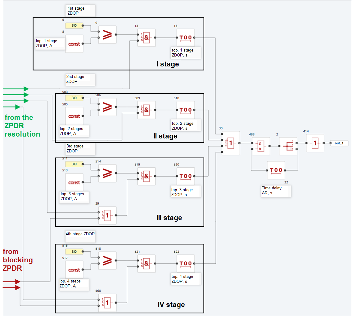
Fig. 6 Implementation of the four-stage ZDOP logic

For each stage, a comparison of the measured current \(3I_0\) with the setting is implemented (e.g., for stage 1, this is block №5, blocks №8 and №9), a check for the presence of a signal from the ZPDR (blocks №13, №509, №519, №521 for the respective stages), and a time delay (blocks №15, №510, №520, №522 for the respective stages). Signals from each stage go to the block №30 Logical OR, and if at least one stage operates, a trip signal for the circuit breaker is generated. The SR latch block №488 and the Switch-on delay block №22 are used to model the action of automatic re-enablement (AR) of the line.

Note

This model implements a primitive AR logic without synchronization check, line voltage check, or synchrocheck. In this case, AR is used to model several SC at different points in the scheme over a long simulation time.

2.  Mathematical model for verifying the ZDOP algorithm

 Fig. 7 shows the REPEAT VISION implemented model of a two-machine power system with ZDOP for a 220 [kV] PTL, whose structural diagram is shown in Fig. 1.

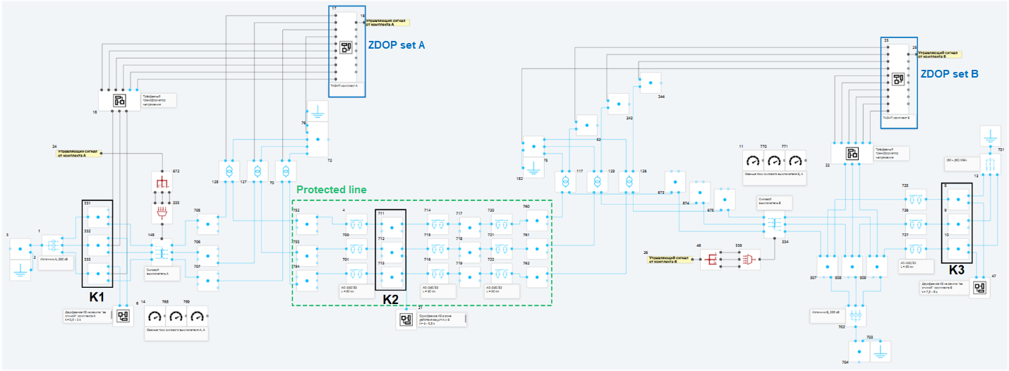
Fig. 7 Scheme for studying ZDOP operation in REPEAT VISION

 To model the given power system, blocks from the Electronics library were used. PTL are represented using Single-phase transmission line blocks, CT - Ideal two windings transformer (transformation ratio 600/5), VT - Ideal three windings transformer (transformation ratio (220/√3) / (0.1/√3)).

 For better perception of the network topology, the ZDOP model is grouped and presented in blocks №17 (set A) and №23 (set B). The model also contains three groups blocks №6, №21, №47, which contain blocks for modeling short circuits, and two groups blocks №16 and №22 with blocks for modeling three-phase VT. Fig. 8 shows one of the models of a three-phase VT.

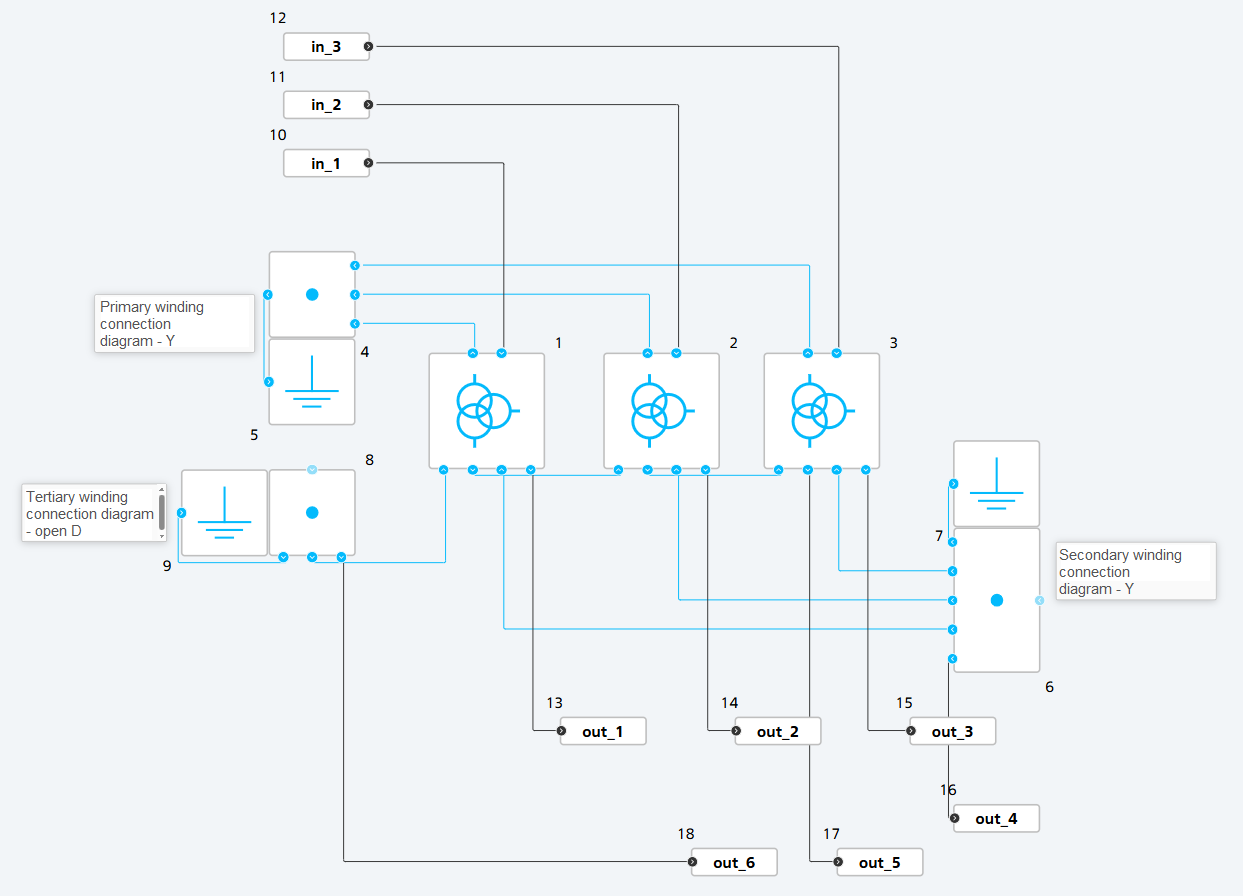
Fig. 8 Model of a three-phase voltage transformer

The primary and secondary windings are connected in a “star” configuration, and the tertiary winding is connected in an “open delta”. As noted earlier, the latter configuration allows measuring the zero-sequence voltage between the two obtained terminals blocks №17 and №18.

 Within this scheme, according to [2], the operating parameters of the protection sets were calculated. The current and voltage pickup settings for the permissive and blocking ZPDR are the same for both protection sets and are equal to 0.34 [A] and 1 [V] in secondary values, respectively. The results of calculating other protection parameters in secondary values are given in tables 3 and 4.

Table 3 Results of calculating the operating parameters for ZDOP Set A

Stage №	Current pickup setting, [A]	Time delay, [s]
I	28.55	0.1
II	17.87	0.75
III	10.81	1.05
IV	9.31	1.35

Table 4 Results of calculating the operating parameters for ZDOP Set B

Stage №	Current pickup setting, [A]	Time delay, [s]
I	17.66	0.1
II	9.25	0.75
III	5.46	1.05
IV	5.4	1.35

3.  Implementation of a program for plotting the ZPDR vector diagram

 To analyze the model results using the REPEAT VISION embedded JupyterLite notebook, a program was created, the code of which is provided in the application.

 This program allows plotting vector diagrams for the permissive (\(\phi_{m \hspace{1mm} s}\) = 250°, Fig. 9, a) or blocking (\(\phi_{m \hspace{1mm} s}\) = 70°, Fig. 9, b) zero-sequence power directional relay depending on the value of the angle \(\phi_{m \hspace{1mm} s}\).

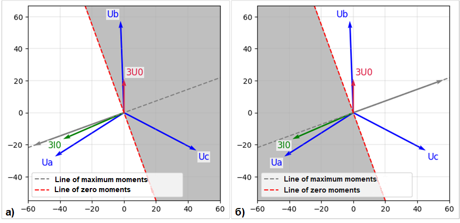
Fig. 9 Vector diagrams of the permissive (a) and blocking (b) ZPDR, plotted using JupyterLite

Hint

• The gray vector on the diagram is plotted at an angle \(\phi_{m \hspace{1mm} s}\) to the voltage vector \(3U_0\). Consequently, the half-plane in which this vector lies is the relay’s operating zone.

• If the current vector \(3I_0\) is positioned as in Fig. 9, the permissive relay will operate.

 For clarity, the relay vector diagrams also include vectors of the secondary phase voltages. To plot them, it is necessary to add Fourier block and Gain block with a gain of 1/√2 to the demo project scheme [DEMO] 220 kv transmission line zero sequence directional overcurrent protection. The addition of blocks for sets A (a) and B (b) is shown in Fig. 10.

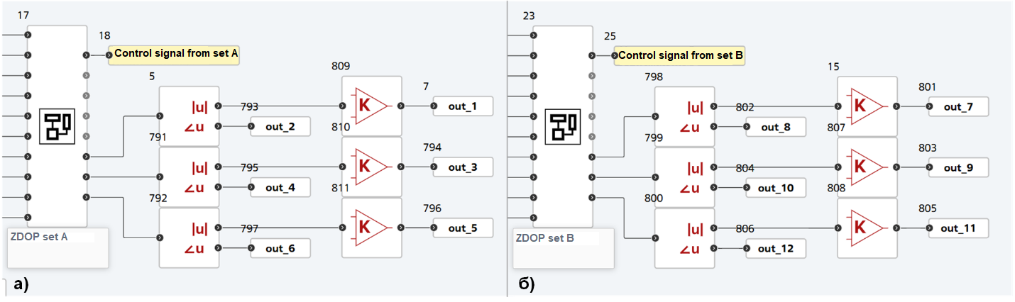
Fig. 10 Adding blocks to the model for plotting vector diagrams

4.  Conducting simulation and evaluating results

 The following computational experiments were performed in the given power system:

1. Two-phase earth SC at points K1 and K3;

2. Single-phase SC at point K2;

3. Phase B break at point K2;

4. Two-phase SC at point K1.

4.1.  Two-phase earth SC

 Fig. 11, 12, 13 and 14 show oscillograms of breaker currents and vector diagrams during a two-phase earth SC in the studied power system model.

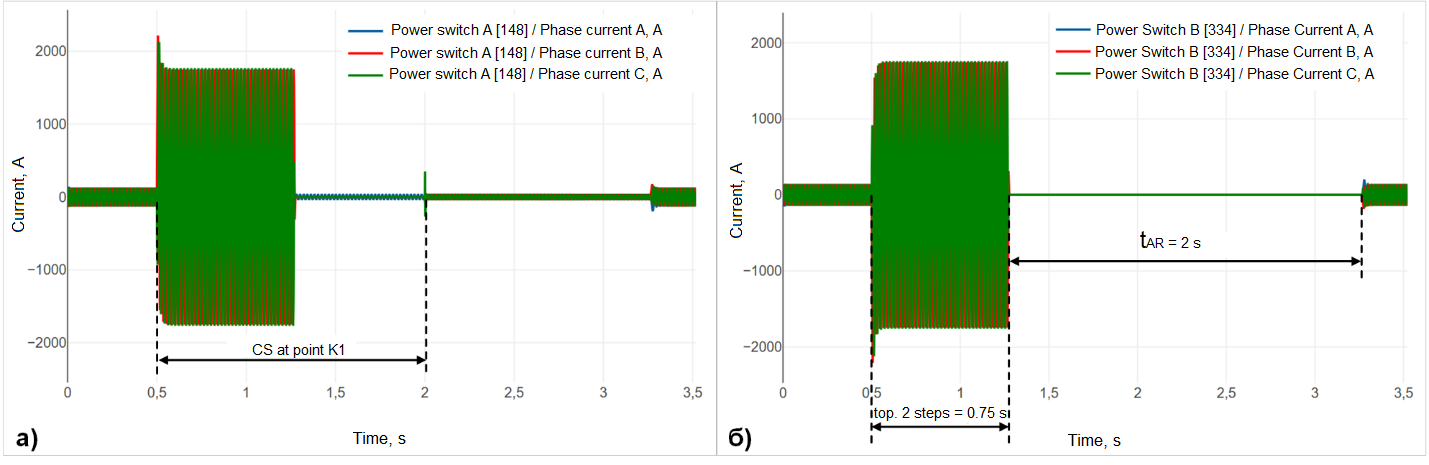
Fig. 11 Oscillograms of breaker currents A (a) and B (b) (two-phase earth SC at point K1)

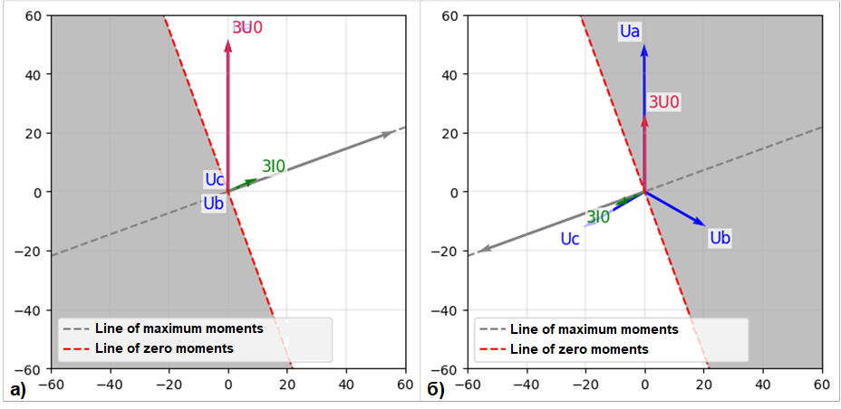
Fig. 12 Vector diagrams of the blocking ZPDR of set A (a) and the permissive ZSPDR of set B (b) (two-phase earth SC at point K1)

The SC at point K1 is within the operating zone of protection set B (see Fig. 1), but it is also located in close proximity to set A. In this case, the blocking relay of set A will operate (Fig. 12, a) and breaker A will not trip. Simultaneously, the permissive ZPDR of set B operates (Fig. 12, b) – breaker B trips due to the operation of stage 2 of protection set B.

Note

The obtained vector diagram of phase voltages (Fig. 12, a) coincides with the theoretical one for a two-phase earth SC in phases B and C, which confirms the correctness of the developed program for plotting the vector diagram.

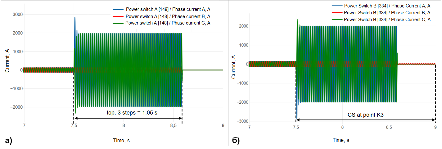
Fig. 13 Oscillograms of breaker currents A (a) and B (b) (two-phase earth SC at point K3)

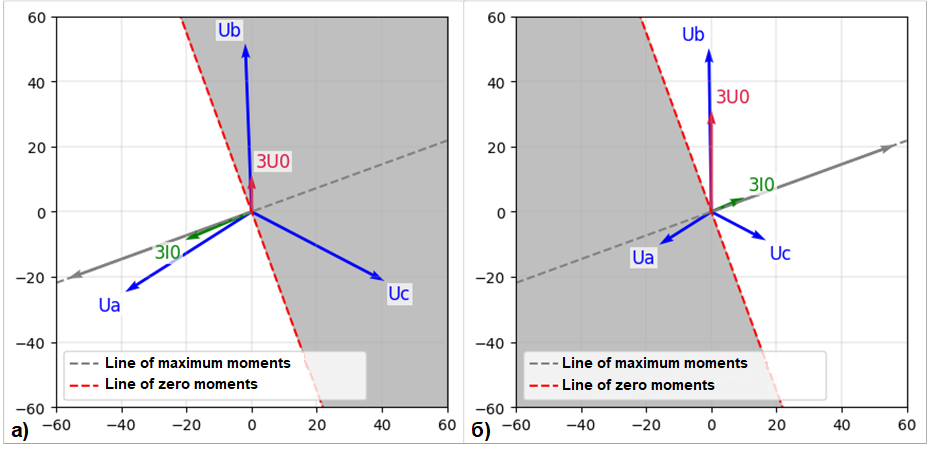
Fig. 14 Vector diagrams of the permissive ZPDR of set A (a) and the blocking ZSPDR of set B (b) (two-phase earth SC at point K3)

The SC point is within the operating zone of set A (see Fig. 1) and is close to set B. However, during an SC at this point, breaker B does not trip due to the operation of the blocking relay of the corresponding set (Fig. 14, b). At the same time, the permissive relay of set A operates (Fig. 14, a), and breaker A trips due to the operation of stage 3 of this protection set.

4.2.  Single-phase SC

 Fig. 15 and 16 show oscillograms of breaker currents and vector diagrams during a single-phase SC at point K2.

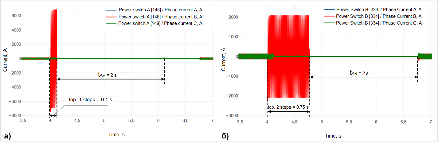
Fig. 15 Oscillograms of breaker currents A (a) and B (b) (single-phase SC at point K2)

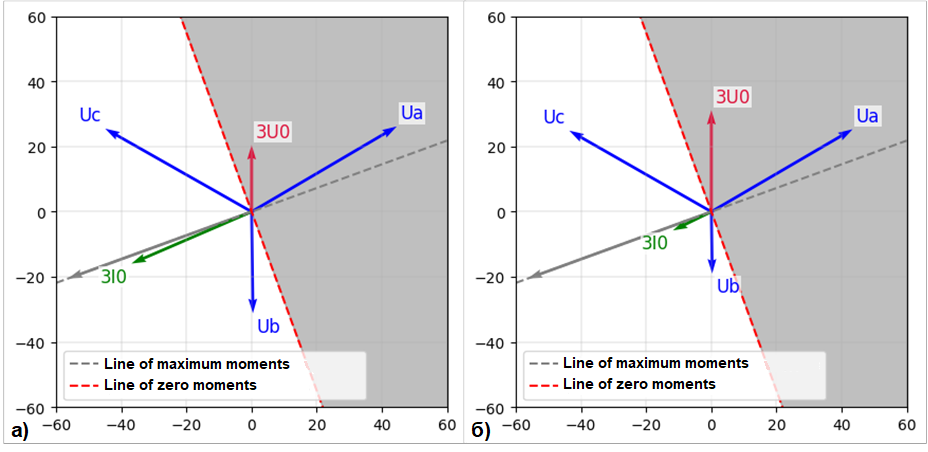
Fig. 16 Vector diagrams of the permissive ZSPDR of set A (a) and the permissive ZSPDR of set B (b) (single-phase SC at point K2)

The SC at point K2 is within the operating zone of both protection sets (see Fig. 1), therefore, both sets operate. Since the fault location is closer to the installation site of protection A, breaker A trips due to the operation of stage 1 of protection set A, and breaker B trips due to the operation of stage 2 of protection set B.

4.3.  Phase break

 To model a phase B break at point K2, a group of blocks was used, which is shown in Fig. 17.

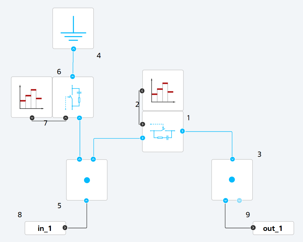
Fig. 17 Blocks for modeling a phase break with earth fault on one side

This experiment considers the case of a phase conductor break at an anchor insulator string [5]. This means that the end of the conductor on one side of the support (in this case, from the side of source A) falls to the ground – causing an earth fault. On the other side of the support (from the side of source B), due to the attachment to the support and tension, the end of the conductor remains suspended – resulting in an open-phase (asymmetrical) operating condition.

 Fig. 18, 19, and 20 show oscillograms of breaker currents, effective values ​​of currents \(3I_0\), and vector diagrams during a phase B break at point K2.

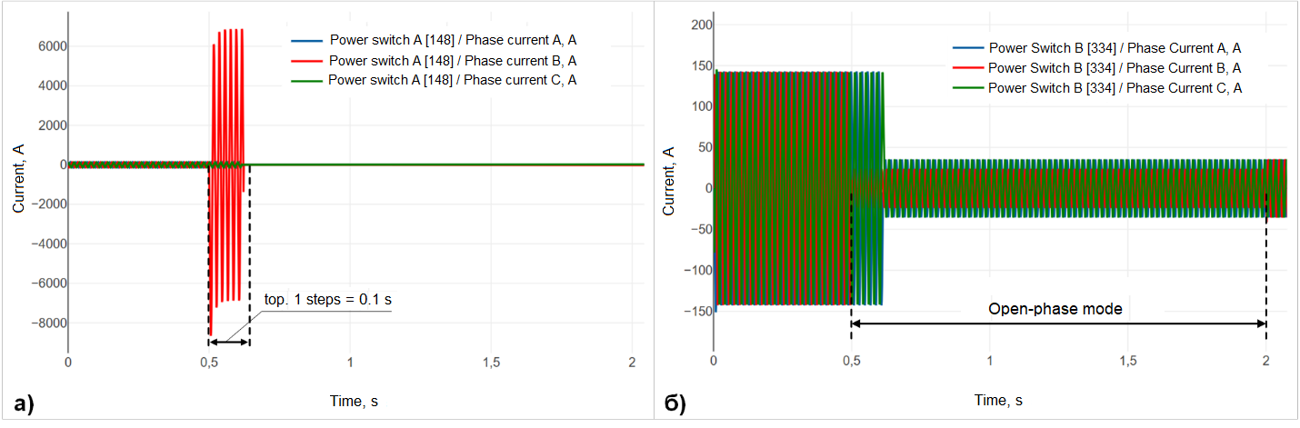
Fig. 18 Oscillograms of breaker currents A (a) and B (b) (phase B break at point K2)

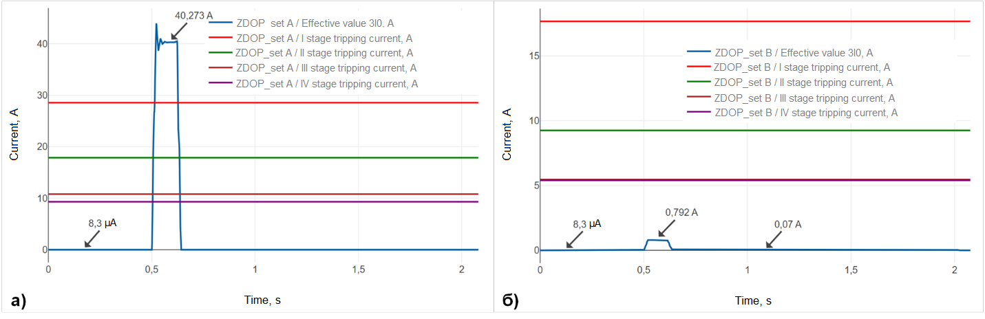
Fig. 19 Effective values ​​of currents \(3I_0\) for sets A (a) and B (b) (phase B break at point K2)

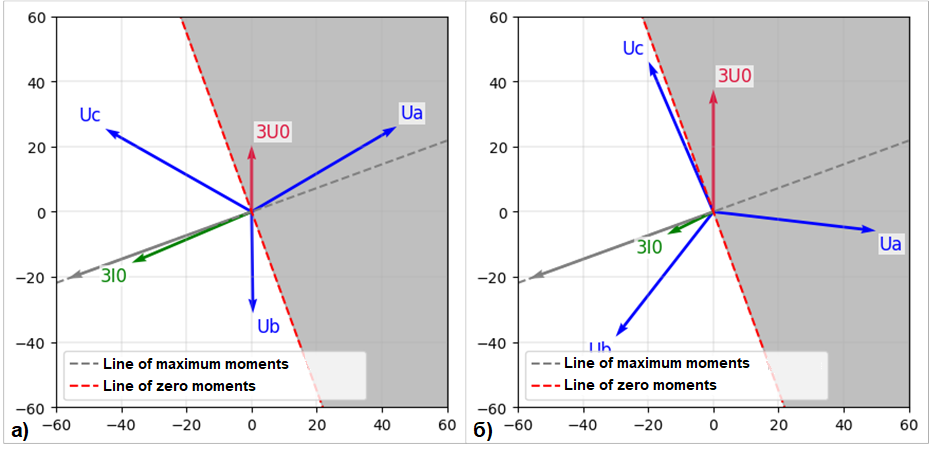
Fig. 20 Vector diagrams of the permissive ZPDR of set A (a) and the permissive ZPDR of set B (b, scale of vectors 3U0 and 3I0 - 20:1) (phase B break at point K2)

Despite point K2 being in the operating area of both protections, only set A operates, since the earth fault is observed from its side – breaker A trips due to the operation of stage 1 of the protection (Fig. 19, a) and the permissive relay (Fig. 20, a). From the side of set B, the permissive ZPDR also operates (Fig. 20, b), however, the magnitude of the zero-sequence current \(3I_0\) is insufficient for the protection stages to operate (Fig. 19, b), so breaker B remains in operation.

4.4.  Two-phase SC

 Fig. 21 – 22 show oscillograms of breaker currents and RMS values of \(3U_0\) and \(3I_0\) during a two-phase SC at point K1.

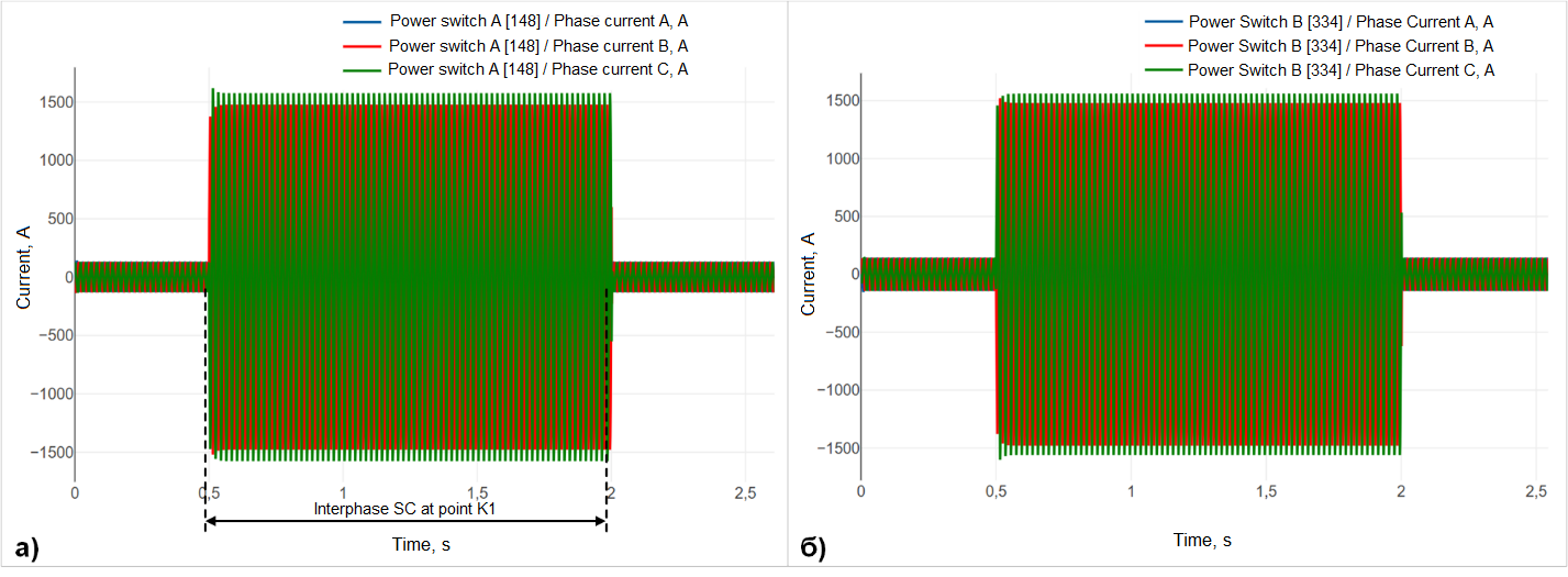
Fig. 21 Oscillograms of breaker currents A (a) and B (b) (two-phase SC at point K1)

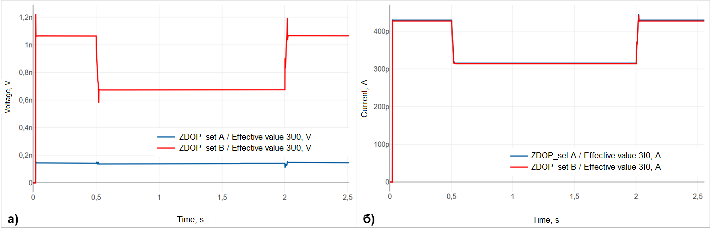
Fig. 22 Effective values ​​of voltages 3U0 (a) and currents 3I0 (b) for sets A and B (two-phase SC at point K1)

The protection sets do not operate because in the case of a phase-to-phase SC, there is no connection to earth and, consequently, no zero-sequence current. Therefore, the values of voltages \(3U_0\) (Fig. 22, a) and currents \(3I_0\) (Fig. 22, b) practically do not change compared to the normal operating mode of the power system.

5.  Conclusions

 This practical guide provided a description and implementation of:

• the operating algorithm of the ZDOP for a 220 [kV] PTL based on the ШЭ2607 016 cabinet by “EKRA”;

• a power system for verifying the protection algorithm;

• a program for plotting vector diagrams of the permissive and blocking ZPDR using the JupyterLite notebook;

• experiments to test the functioning of the developed ZDOP model.

Analysis of the experiment results allows us to conclude that the developed protection model functions correctly. This ZDOP model can be used not only within the presented power system but also in other models for protecting transmission lines with voltage classes of 110 [kV] and above, by saving it as a custom block. If necessary, you can also supplement this model (e.g., complicate the AR logic) or develop your own protection model based on it.

6.  Application

 To use the provided code, it is necessary to:

• specify your API key (variable user) and project number (variable project);

• specify the correct project simulation time (variable t_interval) and the timestamp for plotting the vector diagram (variable TIME_MS);

• assign custom names to the output ports for the RMS values and phases of the zero-sequence current and voltage, and phase voltages when starting the model calculation. In this case, the parameters are set either for set A or for set B.

#Импорт необходимых библиотек
import numpy as np
import matplotlib.pyplot as plt

#Импорт и установка пакета для соединения с рабочей областью в REPEAT VISION
import piplite
await piplite.install('repeat')
from repeat import User, Application, TimeInterval

#Подключение к профилю
user = User ('Ваш API ключ')
app = Application(user)
#Подключение к рабочей области
project = 68828
t_interval = TimeInterval(start = 0, end = 9000) # Время моделирования проекта
model = app.get_exploration_model(project,t_interval)

# Запуск расчёта и получение данных выходных портов из модели
with model as md:
    md.run(model.existing_variables)
    I0A_value = md.get_results('к.A_Действующее значение 3I0, А')
    I0A_phase = md.get_results('к.A_Фаза 3I0, град')
    U0A_value = md.get_results('к.A_Действующее значение 3U0, В')
    U0A_phase = md.get_results('к.A_Фаза 3U0, град')
    Ua_value = md.get_results('к.A_Действующее значение Ua, В')
    Ua_phase = md.get_results('к.A_Фаза Ua, град')
    Ub_value = md.get_results('к.A_Действующее значение Ub, В')
    Ub_phase = md.get_results('к.A_Фаза Ub, град')
    Uc_value = md.get_results('к.A_Действующее значение Uc, В')
    Uc_phase = md.get_results('к.A_Фаза Uc, град')

TIME_MS = 7550  # Время в мс для построения векторов
PHI_MAX_CH = 70  # Угол максимальной чувствительности (250 для разрешающего реле, 70 для блокирующего)
VECTOR_SCALE = 1  # Масштаб для векторов 3U0 и 3I0
X_PLOT_LIMITS = (-60, 60)  # Границы графика по оси X
Y_PLOT_LIMITS = (-60, 60)  # Границы графика по оси Y

# Расчет угла поворота векторов относительно 3U0
gamma = 90 - U0A_phase.iloc[TIME_MS]

# Определение граничного значения для заливки области несрабатывания
if PHI_MAX_CH == 250:
    x_limit = 70
elif PHI_MAX_CH == 70:
    x_limit = -70


def get_vector(length, phase, scale=1, color='black', name=None):
    """Построение вектора с заданными параметрами."""
    angle_rad = np.deg2rad(phase + gamma)
    x, y = length * np.cos(angle_rad), length * np.sin(angle_rad)
    plt.quiver(0, 0, x, y, angles='xy', scale_units='xy', scale=scale,
               color=color)

    if name:  # Определение оптимального размещения подписи вектора
        offset = 1.1
        ha_options = ['left', 'right']
        va_options = ['bottom', 'top']

        # Выравнивание подписи по положению вектора
        ha = ha_options[int(np.cos(angle_rad) < 0)]
        va = va_options[int(np.sin(angle_rad) < 0)]

        # Смещение подписи
        offset_x = offset if ha == 'left' else -offset
        offset_y = offset if va == 'bottom' else -offset

        plt.text(x / scale + offset_x, y / scale + offset_y, name,
                 color=color, fontsize=12, va=va, ha=ha,
                 bbox=dict(facecolor='white', alpha=0.7, edgecolor='none',
                           pad=1))


def plot_line(angle_deg, vector_length=60, linestyle='--', color='gray',
              label=None):
    """Построение прямой и вектора с заданным углом."""
    angle_rad = np.deg2rad(U0A_phase.iloc[TIME_MS] + angle_deg + gamma)
    x_line = np.linspace(*X_PLOT_LIMITS, 120)
    y_line = np.tan(angle_rad) * x_line
    plt.plot(x_line, y_line, linestyle=linestyle, color=color, label=label)

    if vector_length:  # Построение вектора, сонаправленного с линией
        x_vec, y_vec = vector_length * np.cos(
            angle_rad), vector_length * np.sin(angle_rad)
        plt.quiver(0, 0, x_vec, y_vec, angles='xy', scale_units='xy', scale=1,
                   color=color)


# Построение линий максимального и минимального моментов
plot_line(-PHI_MAX_CH, label='Линия максимальных моментов')
plot_line(-PHI_MAX_CH - 90, vector_length=None, color='red',
          label='Линия нулевых моментов')

# Заливка области несрабатывания реле
x_line = np.linspace(*X_PLOT_LIMITS, 120)
y_line = np.tan(
    np.deg2rad(U0A_phase.iloc[TIME_MS] - PHI_MAX_CH - 90 + gamma)) * x_line
plt.fill_between(x_line, y_line, x_limit, alpha=0.5, color='gray')

# Построение векторов фазных напряжений
data = {
    'Ua': {'value': Ua_value, 'phase': Ua_phase},
    'Ub': {'value': Ub_value, 'phase': Ub_phase},
    'Uc': {'value': Uc_value, 'phase': Uc_phase}
}

for vec_name, vec_data in data.items():
    get_vector(vec_data['value'].iloc[TIME_MS],
               vec_data['phase'].iloc[TIME_MS],
               color='blue',
               name=vec_name)

# Построение векторов 3U0 и 3I0
get_vector(U0A_value.iloc[TIME_MS], U0A_phase.iloc[TIME_MS], VECTOR_SCALE,
           'crimson', '3U0')
get_vector(I0A_value.iloc[TIME_MS], I0A_phase.iloc[TIME_MS], VECTOR_SCALE,
           'green', '3I0')

# Настройка графика
plt.gca().set_aspect('equal', adjustable='box')
plt.xlim(X_PLOT_LIMITS)
plt.ylim(Y_PLOT_LIMITS)
plt.legend(loc='lower left')
plt.grid(linewidth=0.3)
plt.show()

7.  Sources

---

[1] (1,2)

Handbook of electrical network design / edited by D. L. Faibisovich. - 4th edition, revised and enlarged. - M.: ENAS, 2012. - 376 p.: ill.

[2] (1,2,3)

Guidelines for calculating and selecting the parameters for setting up backup current protection for power transmission lines of 110 kV and higher. Approved by the order of JSC SO UES No. 61r dated 10.05.2023. URL: https://www.so-ups.ru/functioning/tech-base/tech-standards/.

[3]

EKRA.656453.183 RE. Line protection and circuit breaker control automation cabinet. – Cheboksary: ​​OOO NPP EKRA, 2016. – 164 pp.

[4]

Fedotov, V.P. Design of microprocessor protection of elements of electrical networks with voltage of 110-220 kV: teaching aid / V.P. Fedotov, S.S. Staroselnikov, L.A. Fedotova. - 2nd ed., revised. and add. - Ekaterinburg: Publishing house of the Ural. University, 2018. - 268 p.

[5]

Lastovkin, V. VL 110-220 kV. Diagnostics of phase break under operating voltage // Information and reference publication “Electrical Engineering News”. - No. 2, 2010. URL: http://news.elteh.ru/arh/2010/62/05.php.