Development of mathematical model of aircraft pitch angle control system

The aircraft control system (AC) comprises several control circuits to control the speed, altitude and navigation of the aircraft.

The aircraft pitch angle control system is an important circuit for increasing flight stability and contains autopilot controllers responsible for longitudinal movement.

This practical guide comprises:

• The process of developing a mathematical model of the longitudinal movement of the aircraft[1] using the Jython block is given;

• The process of creating a model for controlling the pitch angle of AC using the Automatics block library;

• A Python program is presented for automated adjustment of the coefficients of the PID controller of the pitch angle control system.

1.  Mathematical model of aircraft longitudinal motion

This practical guide will simulate the longitudinal motion of a civilian aircraft, schematically represented in the figure below[1].

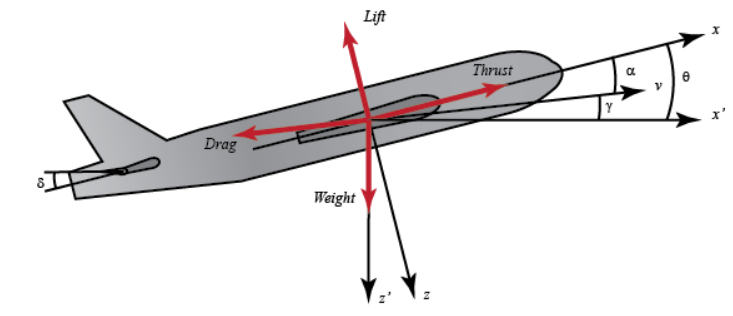
Civil aircraft coordinate system

The following designations are adopted in the figure above.

Designations	Description
Black coordinate axes	Coordinate axes: \(\mathbf{x, z}\) are the axes of the related CS; \(\mathbf{x', z'}\) are the axes of the earth CS.
Red force vectors	Main forces acting on AC in longitudinal motion: Thrust - traction force, Lift - lifting force, Drag - resistance force, Weight - - weight AC.

The following assumptions are used in the civilian aircraft model:

1. AC is in steady state at constant altitude and speed;

2. Change of pitch angle does not result in change of aircraft speed.

The accepted assumptions allow us to form a model of longitudinal motion AC in the form of a system of equations (1).

(1)\[\begin{split}\left\{ \begin{aligned} \dot{\alpha} &= \mathrm{\mu} \cdot \mathrm{\Omega} \cdot \Bigg[ -\left(\mathrm{C}_{\mathrm{L}} + \mathrm{C}_{\mathrm{D}}\right) \cdot \mathrm{\alpha} + \frac{q}{\left(\mathrm{\mu} - \mathrm{C}_{\mathrm{L}}\right)} - \left(\mathrm{C}_{\mathrm{W}} \cdot \sin\mathrm{\gamma}\right) \cdot \mathrm{\theta} + \mathrm{C}_{\mathrm{L}} \Bigg]; \\ \dot{q} &= \frac{\mathrm{\mu} \cdot \mathrm{\Omega}}{2 \cdot i_{yy}} \Bigg[ \left(\mathrm{C}_{\mathrm{M}} - \mathrm{\eta} \cdot \left(\mathrm{C}_{\mathrm{L}} + \mathrm{C}_{\mathrm{D}}\right)\right) \cdot \alpha + \left(\mathrm{C}_{\mathrm{M}} + \mathrm{\sigma} \cdot \mathrm{C}_{\mathrm{M}} \cdot \left(1 - \mathrm{\mu} \cdot \mathrm{C}_{\mathrm{L}}\right)\right) \cdot q \\ &\quad + \left(\mathrm{\eta} \cdot \mathrm{C}_{\mathrm{W}} \cdot \sin\mathrm{\gamma}\right) \cdot \delta \Bigg]; \\ \dot{\theta} &= \Omega \cdot q. \end{aligned} \right.\end{split}\]

The following factors are used in the (1) equation:

(2)\[\begin{split}\begin{aligned} \mu &= \frac{\rho \cdot S \cdot \dot{c} }{4 \cdot m}; \\ \Omega &=\frac{2 \cdot U}{\dot{c}}; \\ \sigma &=\frac{1}{1+\mu \cdot C_{L}}; \\ \eta &=\mu \cdot \sigma \cdot C_{M}. \end{aligned}\end{split}\]

The following designations are adopted in the (1) and (2) equations:

Designation	Description
\(\alpha\)	Angle of attack shown in Figure above
\(\dot{\alpha}\)	First order derivative of angle of attack
\(\theta\)	Pitch angle (see figure above)
\(\dot{\theta}\)	First order derivative of pitch angle
\(q\)	Pitch angular velocity
\(\dot{q}\)	First order derivative of pitch angular velocity
\(\delta\)	Angle of elevator (see Figure above)
\(\rho\)	Air density
\(S\)	Wing area
\(\dot{c}\)	Average chord length
\(m\)	Mass of AC
\(U\)	Steady state flight speed
\(C_{T}\)	Traction coefficient
\(C_{D}\)	Resistance coefficient
\(C_{L}\)	Lifting force coefficient
\(C_{W}\)	Weight factor
\(C_{M}\)	Pitch torque coefficient
\(\gamma\)	Flight direction angle (see figure above)
\(i_{yy}\)	Normalized moment of inertia

In the case of using the coefficients of a civilian aircraft, the equation (1) takes the following form (3).

(3)\[\begin{split}\left\{ \begin{aligned} \dot{\alpha} &= -0.313 \cdot \alpha + 56.7 \cdot q + 0.232 \cdot \delta; \\ \dot{q} &= -0.0139 \cdot \alpha -0.426 \cdot q + 0.0203 \cdot \delta; \\ \dot{\theta} &= 56.7 \cdot q. \end{aligned} \right.\end{split}\]

For the subsequent implementation of the longitudinal motion model AC in the Jython block, a matrix representation of the equation (3) is required.

(4)\[\begin{split}\left[\begin{array}{c}\dot{\alpha} \\ \dot{q} \\ \dot{\theta} \end{array}\right] = \left[\begin{array}{ccc} -0.313 & 56.7 & 0\\ -0.0139 & -0.426 & 0 \\ 0 & 56.7 & 0 \end{array}\right] \cdot \left[\begin{array}{c} \alpha \\ q \\ \theta \end{array}\right]+\left[\begin{array}{c} 0.232 \\ 0.0203 \\ 0 \end{array}\right] \cdot \delta \end{split}\]

The mathematical model of the control system adjusts the pitch angle, so the output expression for the control system is (5).

(5)\[\begin{split}y=\left[\begin{array}{ccc}0& 0& 1\end{array}\right] \cdot \left[\begin{array}{c}\alpha \\ q\\ \theta \end{array}\right] \end{split}\]

In order to solve the problem of determining the pitch angle \( heta\), \(\dot{ heta}\) derivative of the pitch angle is integrated by the numerical Euler method according to the equation (6).

(6)\[\begin{split}\left[\begin{array}{c}\alpha _{t+\mathrm{\Delta }t}\\ q_{t+\mathrm{\Delta }t}\\ \theta _{t+\mathrm{\Delta }t}\end{array}\right]=\left[\begin{array}{c}\alpha _{t}\\ q_{t}\\ \theta _{t}\end{array}\right]+\mathrm{\Delta }t\cdot \left[\begin{array}{c}\dot{\alpha }\\ \dot{q}\\ \dot{\theta }\end{array}\right]\end{split}\]

The following designations are accepted in the equation (6):

Designation	Description
\(\Delta t\)	Integration step. The step value used to configure the project is shown in the table below.
\(\alpha_{t}\)	Angle of attack value in previous step
\(q_{t}\)	Value of pitch angular velocity at the previous step
\(\theta_{t}\)	Pitch angle value in previous step
\(\alpha_{t + \Delta t}\)	Value of angle of attack at current step
\(q_{t + \Delta t}\)	Value of pitch angular velocity at the current step
\(\theta_{t + \Delta t}\)	Pitch angle value at current step

2.  Overview of the demonstration model of aircraft pitch angle control in REPEAT VISION application

An example of an aircraft pitch angle control model is available in the set of demonstration projects of the REPEAT VISION application. Next, let’s analyze this example, which will help us describe all the necessary steps to implement the AC pitch angle control model on the REPEAT VISION platform.

In the REPEAT VISION application, add the [DEMO] project Aircraft pitch angle control system project from the Demo projects folder and open it for further review.

Demonstration project of an aircraft pitch angle control system

In the demo project shown in figure above, use the following settings.

Setup	Value
Real-time synchronization	Off
Simulation time	40 \([s]\)
Integration step	1 \([ms]\)
Sampling rate	100 \([ms]\)

2.1.  Implementation of the AC longitudinal motion model

Two blocks are used to calculate the pitch angle \( heta\) in the longitudinal motion model AC:

Block	Project Block №	Model assignment
Constant	Block №1	Required for \( heta\) assignment, pitch angle setpoint (see AC diagram), by \(0.2 [rad]\) value
Jython	Block №8	Required to directly implement the (3) equation using the matrix form (4)

The longitudinal motion model AC is implemented in the Python programming language using the Jython block.

In order to review the longitudinal motion model of AC, it is required to click on the button Edit block code in the properties of block №8 Jython.

In the Jython block, three tabs are available for implementing the Python code of the program.

Initialization

This step is coded once before the simulation to prepare for the calculation process. At this stage, you need to perform:

1. Import of required libraries;

2. Create program items for which you want to save the state between the execution of integration steps in the calculation process;

3. Create the necessary functions and classes for the next call at the simulation stage in Calculation code.

Calculation code

Code of this stage is executed at each integration step from the beginning of the calculation to its stop. The following is necessary at this stage:

1. Call functions and methods of Python classes of the program responsible for simulation;

2. Use in values of the input ports of the Jython block and return the results to out output ports of the Jython block;

Items created within the calculation code* do not retain their state after the integration step is completed.

If your items need to maintain a state between integration steps, then they should be created and configured at the initialization stage and then used in the calculation code.

End

The code of this stage is executed once when the calculation is stopped.

At the end of the calculation, the data of Python program items can be processed, the state of which between the implementation of the integration steps was required to be saved in the calculation process.

Next, in the text editor of the Jython block code, one needs to go to the Initialization tab to analyze the preparation code and configure the AC longitudinal motion model.

As part of the initialization, a matrix and a coefficient vector are created, and a function is implemented to solve the system of equations (4) in order to further obtain a vector of angular values of attack and pitch during the longitudinal movement of the aircraft at the next stage of simulation.

Initialization

from org.apache.commons.math3.linear import Array2DRowRealMatrix, ArrayRealVector


COEFF_MATRIX = Array2DRowRealMatrix([
    [-0.313, 56.7, 0.],
    [-0.0139, -0.426, 0.],
    [0., 56.7, 0.]
])
COEFF_VECTOR = ArrayRealVector([0.232, 0.0203, 0.]) 
STATE_VECTOR = ArrayRealVector([0., 0., 0.])
INTEGRATION_STEP = 1e-3

def calculate_angles(input_value):
    """
    Функция выполняет расчёт вектора угловых значений атаки и тангажа
    при продольном движении ЛА.

    Входным аргументом input_value функции является 
    вещественное значение угла руля высоты.
    """

    # В левой части выполняется 
    # умножение матрицы коэффициентов на вектор состояния
    left_part = COEFF_MATRIX.operate(STATE_VECTOR)

    # В правой части выполняется 
    # умножение вектора коэффициентов на значение угла руля высоты 
    right_part = COEFF_VECTOR.mapMultiply(input_value)
    
    # В результате выполняется сложение левой и правой частей
    angles = left_part.add(right_part)

    return angles

• Line 1. Import the required data structures from the linear algebra module of the Apache Commons Math library. The Array2DRowRealMatrix matrix and the ArrayRealVector vector of real values will be used later to calculate the system of equations (3) represented in the matrix form (4);

• Lines 4, 8. Creating a matrix object of coefficients of equations (4) of the longitudinal movement of a civil aircraft. The matrix will further be used in the calculate_angles function;

• Line 9. Creating a coefficient vector on the right side of equations (4);

• Line 10. Creating a model state vector with initial values for angle of attack \(\alpha\), pitch angular velocity \(q\) and pitch angle \( heta\). Further, at the simulation stage, the STATE_VECTOR vector will update the state at the end of each integration step;

• Line 11. Creating the value of the integration step (in seconds) previously specified when configuring the project;

• Lines 13, 33. Creating the calculate_angles function in order to solve the system of equations (4) for calculating the vector of angular values of attack and pitch during the longitudinal movement of the aircraft. The input_value function argument is the real value \(\delta\) of the elevator angle (see figure above).

Next, in the text editor of the Jython block code, one needs to go to the Calculation code tab to analyze the stage of the program that is running at the simulation stage.

As part of the simulation stage, a vector of angular values of attack and pitch is calculated at each integration step from the initial simulation time to the stop of the calculation. This state vector is updated using the explicit Euler method.

As a result of each integration step, the actual value of pitch angle is generated for its subsequent use by the control system.

Calculation code

# Выполняется расчёт вектора угловых значений атаки и тангажа
# при продольном движении ЛА
angles = calculate_angles(in_1)

# Обновляется вектор состояния с учётом шага интегрирования
angles_step = angles.mapMultiply(INTEGRATION_STEP)
STATE_VECTOR = STATE_VECTOR.add(angles_step)

# На выходной порт передаётся значение угла тангажа 
# по индексу №2 вектора состояния
out_1 = STATE_VECTOR.getEntry(2)

• Line 3. At each integration step equal to \(1 [ms]\), the vector of angular values of attack and pitch is calculated for the current input value {math} \delta of the elevator angle obtained from the {bdg-dark-line}in_1` item of the input port;

• Lines 6, 7. Updating STATE_VECTOR state vector using explicit Euler method.

• Line 11. As a result of executing the Calculation code, an item out_1 of the output port of the Jython block is created at each integration step, into which the current value of the pitch angle \( heta\) is output.

2.2.  Implementation of aircraft pitch angle control system model

The following blocks are used to simulate the control system itself:

Block	Project Block №	Model assignment
Signal difference (Controller error)	Block №2	Subtracts the calculated value \( heta\)of the model pitch angle implemented in the Jython block from the pitch angle setpoint. The difference is transmitted to the PID controller of the control system through splitter №3.
Branching	Block №3	Transmits a signal from the comparator to transfer links №4, 5, 6
Gain	Block №4	Required to adjust the proportional coefficient until an acceptable signal growth rate is achieved
Integrating block (Time domain integration)	Block №5	Designed to amplify the integral coefficient to reduce the steady-state error
Differentiation block with characteristic time	Block №6	Required to adjust the differential coefficient to reduce critical oscillations in the system
Addition (linear combination)	Block №7	Summarizes the results of the transmission links within the PID controller implementation

In block №6 of differentiating link, the Таu parameter is assigned a small time value equal to \(1\mathrm{e}{-5}\).

The project contains a set of global variables according to the table below.

Parameter	Global variable name	Applies to block
Proportional link coefficient	PROPORTIONAL_COEFF	block №4
Integrating link factor	INTEGRAL_COEFF	block №5
Differentiating link factor	DIFFERENTIAL_COEFF	block №6

Hint

Global variables allow conveniently controlling project settings in the process of customizing and debugging the model.

Also, global variables are necessary for the interaction of external user programs with the model implemented on the REPEAT VISION platform. For more information on interaction with the REPEAT VISION platform, see tutorial section.

Results of the first simulation of aircraft pitch angle control system

In order to obtain the first simulation results, one shall assign the values to the global PID controller variables according to the table below.

Parameter	Global variable name	Value
Proportional link coefficient	PROPORTIONAL_COEFF	1.0
Integrating link factor	INTEGRAL_COEFF	0.0
Differentiating link factor	DIFFERENTIAL_COEFF	0.0

Next, start the project for calculation and create a new chart in the Visualization panel.

Add the out_1 port parameter Jython of block №8 to the chart to analyze the values of \( heta\) pitch angle.

(png, hires.png)

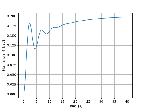
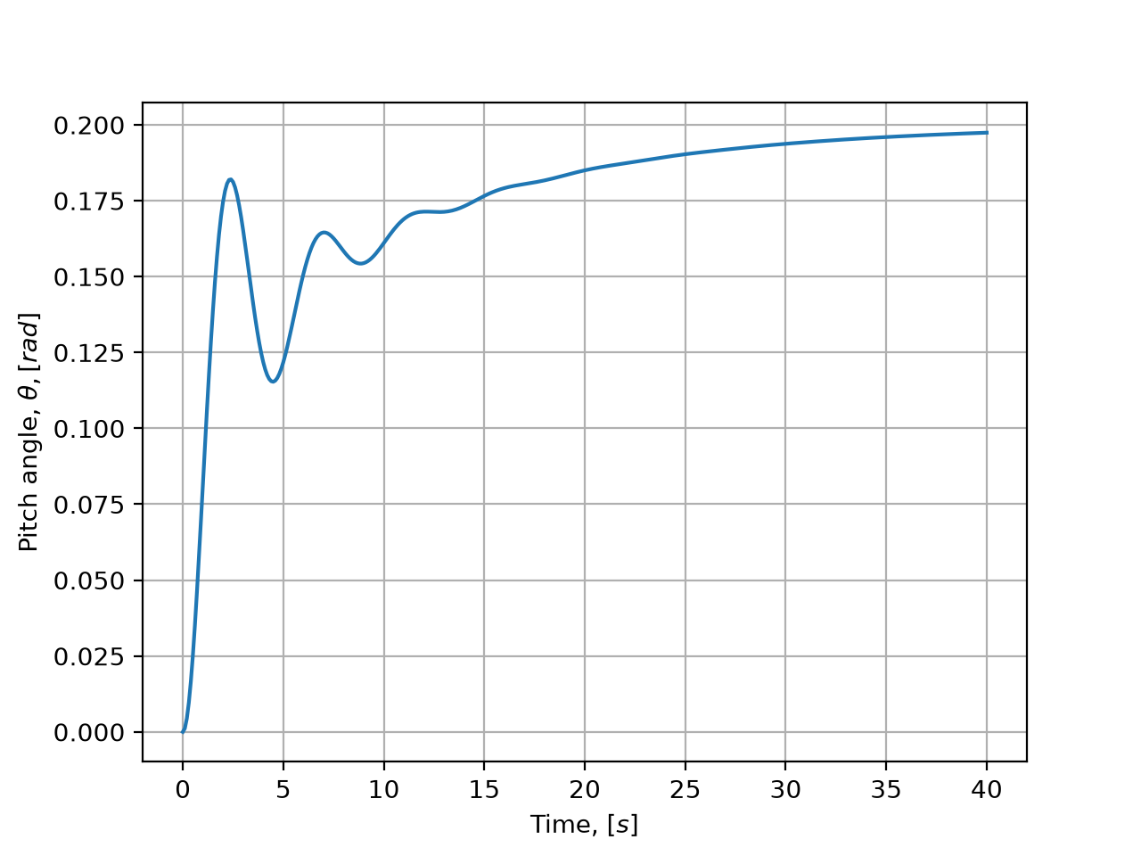
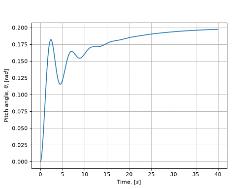
Dependence of change in pitch angle on time.

The following designations are taken in the chart above.

Lines	Description
Blue line	Dependence of change in pitch angle \( heta [rad]\) on time \([s]\)

The following criteria of response quality are used to analyze the calculation results and adapt the model of the pitch angle control system AC:

№	Criterion	Maximum allowable value
1	Overshoot \(\sigma\)	0.15
2	Adjustment time \(t_{contr}\) with precision corridor of 0.05	\(10 [s]\)
3	Relative error of steady value of pitch angle \(\varepsilon_{S}\)	0.05

Response quality criteria are determined by the expressions (7).

(7)\[\begin{split}\begin{aligned} \varepsilon_{S} &= \frac{\theta_{S} - \theta_{T}}{\theta_{T}} \\ \sigma &= \frac{\theta_{max} - \theta_{S}}{\theta_{S}} \end{aligned}\end{split}\]

The following designations are adopted in the equation (7):

Designation	Description
\(\varepsilon_{S}\)	Relative error of steady pitch angle value
\(\theta_{S}\)	Design steady pitch angle value \( heta\)
\(\theta_{T}\)	Pitch angle setpoint \( heta = 0.2 [rad]\)
\(\sigma\)	Overshoot
\(\theta_{max}\)	Maximum design pitch angle \( heta\)

The control time criterion \(t_{contr}\) with an accuracy corridor of 0.05 is shown in chart below.

(png, hires.png)

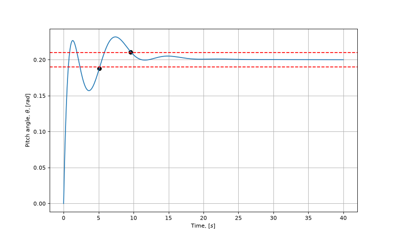
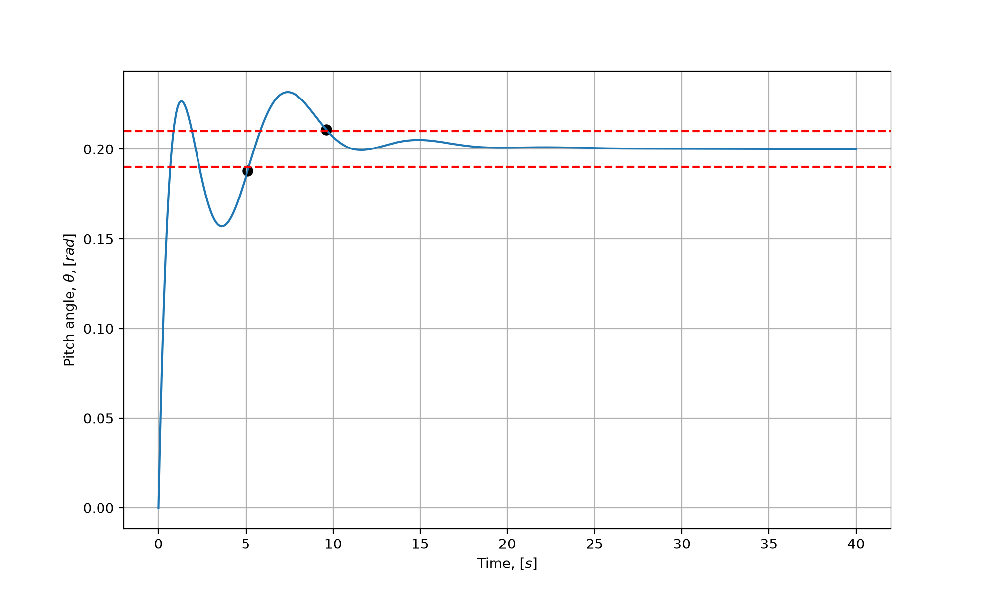
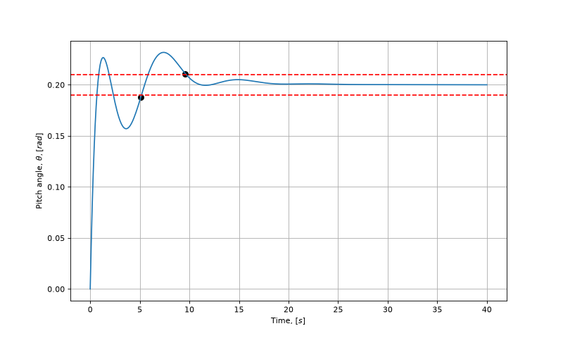
Control time criterion with accuracy corridor.

Next, it is necessary to analyze the results of calculating the model of the aircraft pitch angle control system made with the input data given in Table above.

The following criteria values are obtained using the expression (7): \(\sigma = 0\), \(t_{contr} = 22.2 [s]\), \(\varepsilon_{S} = -0.012\).

Criteria of quality failed. The model requires adjustment of the control system coefficients.

Tip

The empirical method of adjusting the coefficients of the control system model can take a long working time.

Use the optimizer to reduce the effort required to adjust the control system coefficients and to improve the accuracy of model adaptation.

The automated process of aircraft pitch angle control system model adaptation through optimization problem solution is given in the next section.

2.3.  Adaptation of aircraft pitch angle control system model

The following blocks are used in the project to solve the optimization problem of determining the optimal coefficients of PID controller of AC pitch angle control system:

Block	Project Block №	Model assignment
Output port	block №10	Required for transmission of calculation results to Python program \( heta\) of AC pitch angle

In block №10, the user name pitch is assigned for the convenience of obtaining the calculation results.

Also, to solve the optimization problem, the project uses global variables prepared earlier.

Global variables are used by the optimizer as parameters of the objective function for solving the optimization problem.

See also

Detailed information on setting up a REPEAT VISION platform project to interact with external programs can be obtained in the tutorial section.

Setting an optimization task

Optimization problem Minimize a target function of (8) form

(8)\[F(K_p, K_i, K_d) = w_{\sigma} \cdot \sigma^2 + w_S \cdot \varepsilon_S^2 + w_{t_{рег}} \cdot t_{рег}^2,\]

The (8) function uses the following designations \( w_{\sigma}, w_S, w_{t_{contr}} \) - weight coefficients for overshoot, stationary error and adjustment time, allowing taking into account these error components in different ways.

Minimizing the target function means reducing errors and achieving the parameters of the required operation of the control system.

Additionally, after optimization, the requirements of model quality criteria are checked:

\[\sigma \leq 0.15, \quad \varepsilon_S \leq 0.05, \quad t_{рег} \leq 0.4. \]

The following restrictions on variables are used when solving an optimization problem:

(9)\[K_p, K_i, K_d \in [0, 2],\]

As a result, we have an optimization problem:

(10)\[\begin{split}\left\{ \begin{aligned} & \min_{K_p, K_i, K_d} F(K_p, K_i, K_d), \\ & \sigma \leq 0.15, \\ & \varepsilon_S \leq 0.05, \\ & t_{рег} \leq 0.4, \\ & K_p, K_i, K_d \in [0, 2]. \end{aligned} \right.\end{split}\]

Implementation of optimization problem on the REPEAT VISION platform

First open notebook and create a script in a new notebook to connect to the model through the REPEAT VISION platform.

Next, in the first cell, add the Python boot code repeat package, which is necessary for interacting with the REPEAT VISION platform and for solving the optimization problem.

import piplite
await piplite.install("repeat")

In the next cell, import the Python packages needed to prepare the data, process the calculation results, and then visualize the charts in order to analyze the solution to the optimization problem.

import numpy as np
import pandas as pd
import scipy.optimize as so
import matplotlib.pyplot as plt

Import the Python repeat package in the following cell.

import repeat as rp

Next, one needs to configure the connection to the REPEAT VISION platform and select a model to solve the optimization problem.

user = rp.User(
  "enter a unique API key from REPEAT VISION user cabinet instead of this comment"
  )
app = rp.Application(user)
# enter a project ID from REPEAT VISION application instead of 12345
project = 12345
model = app.get_exploration_model(project)

Let’s check the connection in the next cell, which can be deleted after debugging the program

print(model, model.existing_variables, sep = "\n")

# ExplorationModel(project = 12345, 
# name = '[DEMO] Система управления углом тангажа самолёта', 
# time_interval = None)
# DIFFERENTIAL_COEFF    0.0
# INTEGRAL_COEFF        0.0
# PROPORTIONAL_COEFF    1.0
# dtype: float64

In the next cell, prepare the response quality criteria in accordance with the expressions (7) and in accordance with the table containing the permissible values of the criteria. Quality criteria are implemented as methods of the СontrolСriterionclass.

When initializing an instance of the class, one needs to transfer the time series of the model calculation result previously received from the REPEAT VISION platform to the __init__() method.

class СontrolСriterion:
    """
    Класс предназначен для определения критериев качества отклика
    
    Parameters
    ----------
    results : pandas.Series
      Временной ряд результата расчёта модели платформы REPEAT VISION
    """
    def __init__(self, results):
        self.results = results
        self.steady_state = results.iloc[-1]
        self.maximum = results.max()
        
    def get_stabilization_time(self, relative_width):
        """
        Метод рассчитывает время регулирования
  
        Parameters
        ----------
        relative_width : float
          Значение доли (от 0 до 0.5) установившейся величины результата расчёта.
  
        Returns
        -------
        stabilization_time : float
          Время регулирования.
        """
        up_bound = 1 + relative_width
        low_bound = 1 - relative_width
        values_up = self.results[self.results > self.steady_state * up_bound]
        values_low = self.results[self.results < self.steady_state * low_bound]
        stabilization_time = np.nanmax([
            values_up.index.max(), 
            values_low.index.max()
        ])
        return stabilization_time

    def get_overshoot_err(self):
        """
        Метод рассчитывает значение перерегулирования
  
        Returns
        -------
        relative_error : float
          Величина перерегулирования.
        """
        relative_error = (
            self.maximum - self.steady_state
        ) / self.steady_state
        
        return relative_error

    def get_steady_state_err(self, target):
        """
        Метод рассчитывает относительную ошибку стационарного значения
  
        Parameters
        ----------
        target : float
          Уставка значения.
  
        Returns
        -------
        relative_error : float
          Относительная ошибка стационарного значения.
        """
        relative_error = (
            self.steady_state - target
            ) / target
        
        return relative_error

• Lines 15, 37. Implementation of the control time calculation method. The value of 0.05 of the accuracy corridor is transferred to the relative_width argument in accordance with the quality criteria table;

• Lines 39, 52. Implementation of the method for calculating overshoot in accordance with the expression (7);

• Lines 54, 72. Implementation of the method for calculating the relative error of a stationary value in accordance with the expression (7). The pitch angle setpoint value is transferred to the target argument in accordance with settings of block №1 Constant.

The methods for calculating the quality criteria of the СontrolСriterion class will be further used when implementing the target objective_kernel function.

def objective_kernel(angles, target, relative_width):
    """
    Целевая функция суммы квадратов нормализованных на единицу
    критериев качества системы управления с учётом весов критериев.

    Parameters
    ----------
    angles : pandas.Series
      Временной ряд результатов расчёта угла [рад] тангажа ЛА.
    target : float
      Величина уставки угла [рад] тангажа ЛА.
    relative_width : float
      Значение доли (от 0 до 0.5) установившейся величины результата расчёта.
  
    Returns
    -------
    y : float
      Значение целевой функции.
    """
    angles.index = angles.index / 1e3 # [мс] в [с]
    сrit = СontrolСriterion(angles)
    overshoot_error = сrit.get_overshoot_err()
    steady_state_error = сrit.get_steady_state_err(target)
    stabilization_time = сrit.get_stabilization_time(relative_width)
    stabilization_time_relative = stabilization_time / angles.index[-1]
    weight_overshoot, weight_steady_state, weight_time = 5, 1, 10
    y = (
        weight_overshoot * overshoot_error**2
        + weight_steady_state * steady_state_error**2
        + weight_time * stabilization_time_relative**2
    )
    return y

• Line 20. The time value is converted from milliseconds to seconds, since the REPEAT VISION platform API forms time series with a time dimension of \([ms]\);

• Lines 22, 24. Calculation of controller quality criteria in accordance with expressions (7);

• Line 25. Normalization of the time-per-unit criterion for use in the (10) objective function;

• Line 26. Creation of constant values of criteria weights for successful solution of optimization problem. The weights of the criteria are empirically assigned by the engineer;

• Lines 27, 31. Computing the target function value according to (10).

In the next cell, one needs to prepare the auxiliary function run() to interact with the REPEAT VISION platform to transmit the values of global model variables to variables and then obtain the results of calculating the time series of pitch angle values.

def run(model, variables):
    """
    Функция подготовки временного ряда результатов одного расчёта
     
    Parameters
    ----------
    model : repeat.ExplorationModel
      Экземпляр класса ExplorationModel для взаимодействия с платформой REPEAT VISION.
    variables : pandas.Series
      Набор глобальных переменных модели.
  
    Returns
    -------
    angles : pandas.Series
      Временной ряд результатов расчёта угла [рад] тангажа ЛА с 0 до 40 [с].
  
    """
    with model as md:
        md.run(variables)
        angles = md.get_results("pitch",  
                                rp.TimeInterval(start = 0, end = 40.0e3))
        
    return angles

The run() function returns the time series of pitch angle values from block №10 Output port. An example of the calculation results is given in the chart of the results of the first calculation.

In the next cell, an auxiliary function is prepared to interact with the scipy package interface for the further process of solving the optimization problem.

def objective(pid_terms, model, target, relative_width):
    """
    Вспомогательная внешняя функция для целевой функции objective_kernel и
    и для функции run. Функция objective обеспечивает взаимодействие
    непосредственно с оптимизационными алгоритмами пакета scipy

    Parameters
    ----------
    pid_terms : numpy.array
      Вектор трёх значений для глобальных переменных модели REPEAT VISION.
    model : repeat.ExplorationModel
      Экземпляр класса ExplorationModel для взаимодействия с платформой REPEAT VISION.
    target : float
      Величина уставки угла [рад] тангажа ЛА.
    relative_width : float
      Значение доли (от 0 до 0.5) установившейся величины результата расчёта.
  
    Returns
    -------
    y : float
      Значение целевой функции.
    """
    variables = pd.Series(dict(
        DIFFERENTIAL_COEFF = pid_terms[0], 
        INTEGRAL_COEFF = pid_terms[1],
        PROPORTIONAL_COEFF = pid_terms[2],
    ))
    angles = run(model, variables)
    y = objective_kernel(angles, target, relative_width)
    return y

• Lines 23, 27. A variables pandas.Series item is created, which is required to transfer global variables to the REPEAT VISION platform.

In the next cell, one sets up interaction with the optimizer differential_evolution from the library scipy.optimize and performs the process of solving the optimization problem.

solution = so.differential_evolution(
    objective,
    x0 = [0, 0, 1],
    args = (model, 0.2, 0.05),
    popsize = 8,
    maxiter = 4,
    bounds = so.Bounds(
      [0, 0, 0,], 
      [2, 2, 2,]
                  ),
    seed = 5,
)

# Время расчёта 0:00:02.170500 ...

• Line 2. As the first argument, the objective target function is transferred to the optimizer, which it will minimize;

• Line 3. A list of initial values of global variables is transferred to the following named argument x0 in the strict order used in the objective function: DIFFERENTIAL_COEFF, INTEGRAL_COEFF, PROPORTIONAL_COEFF;

• Line 4. A set of constant parameters and a model item are transferred to the args argument in the order assigned in the objectivefunction: model, target, relative_width;

• Lines 7, 10. The bounds argument is assigned bounds on the area of real values of the search for optimal values of the variables DIFFERENTIAL_COEFF, INTEGRAL_COEFF, PROPORTIONAL_COEFF in accordance with the bounding functions of the target function (9);

• Line 11. The seed argument is assigned a value to ensure reproducibility of the result during debugging of the optimization problem solution.

The initial values of the global variables transferred to the argument x0 are generated empirically by the engineer. The initial value reduces the time to find the optimal solution.

The bounds on the optimal value search area transferred to the bounds argument allow focusing the algorithm on the specified parameter space area. The choice of the search area for optimal values should be based on the physical limitations of the model and the technical requirements for the model.

2.4.  Analysis of the results of the adapted control system model

In order to perform the results analysis, it is necessary to start control system model with optimal values of PID controller coefficients in the next cell to obtain actual results of AC pitch angle change.

variables = pd.Series(dict(
        DIFFERENTIAL_COEFF = solution.x[0], 
        INTEGRAL_COEFF = solution.x[1],  
        PROPORTIONAL_COEFF = solution.x[2]  
))
results = run(model, variables)
results.index = results.index / 1e3
axis = result.plot()
axis.set_xlabel(r"Time, $[s]$")
axis.set_ylabel(r"Pitch angle, $\theta, [rad]$")
axis.grid(True)

• Lines 1, 5. A variables item is created with the optimal values of the global model variables transferred from the x vector of the solution item, which was created in the previous cell based on the result of solving the optimization problem;

• Line 7. Milliseconds are converted to seconds for ease of analysis of the pitch angle time series;

As a result of the operation of the cell above, the chart is plotted below to analyze the current results.

(png, hires.png)

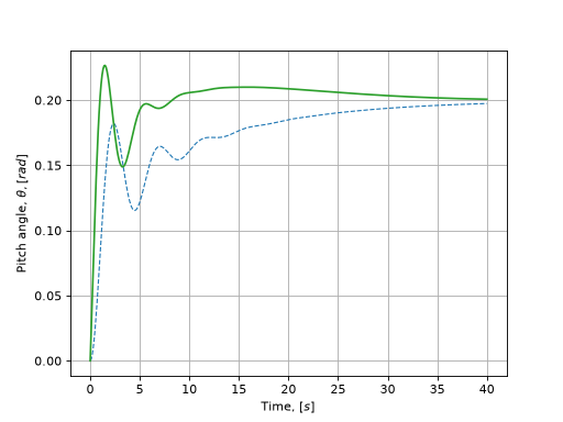
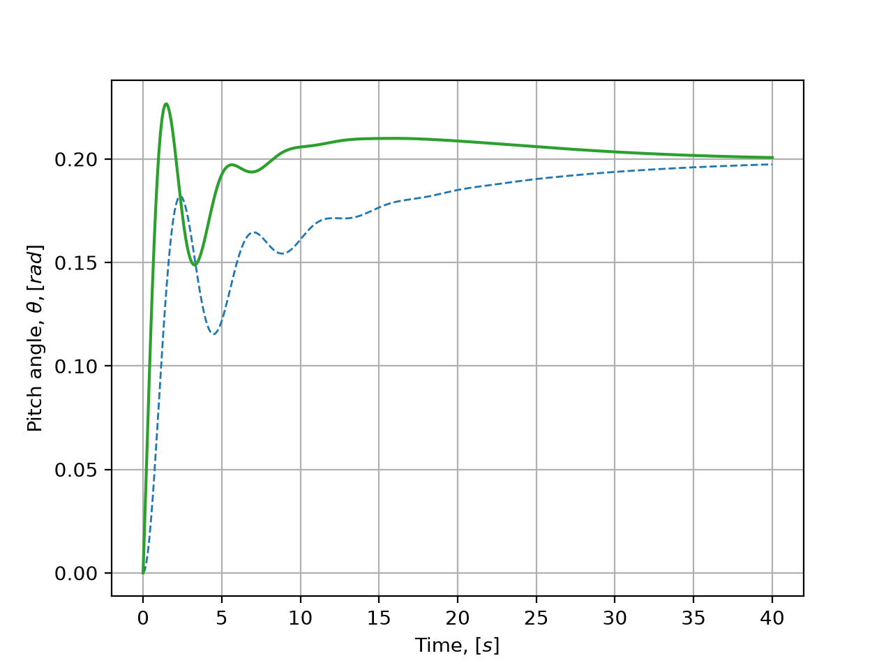
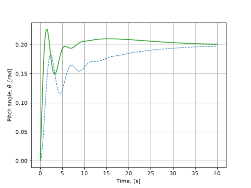
Change in pitch angle over time in an adapted model.

Lines	Description
Blue line	Results of first calculation dependence of pitch angle on time
Green line	Change in pitch angle over time in an adapted model

The results of the control system quality criteria analysis are given in the table below.

№	Criterion	Optimization result	Maximum allowable value
1	Overshoot	0.1293	0.15
2	Adjustment time with precision corridor of 0.05	4.80	\(10 [s]\)
3	Relative error of steady pitch angle value	0.0034	0.05

3.  Conclusions

Within the framework of this practical guide, you managed to master:

• The process of developing a mathematical model of AC longitudinal motion using the Jython;

• The process of creating AC pitch angle control model using the Automatics block library;

• Development process Python program for automated adjustment of the coefficients of PID controller of the pitch angle control system.

4.  References

---

[1] (1,2)

Zakarya Mohammed Motea, Herman Wahid, Junaid Zahid, Swan Htet Lwin and Abbas Musa Hassan, A Comparative Analysis of Intelligent and PID Controllers for an Aircraft Pitch Control System.