

Solving the two-dimensional unsteady-state heat equation with PINN#
External approximation machine learning models allow to consider 2D and 3D dependencies and equations when modeling products and systems on the REPEAT VISION platform.
This practical guide provides a detailed mathematical description of the models of physically informed neural networks (PINN), as well as the ideas from current scientific articles on achieving better convergence of solutions of equations.
You will learn the following skills during this tutorial:
Skills to create and train a ML model to solve the heat transfer problem in a two-dimensional object;
Skills to export machine learning model to ONNX format for further integration into REPEAT VISION platform;
Skills in integrating ML models into the REPEAT VISION platform to use the object model in a system or product design.
1. Task description#
The task is to simulate the dynamics of the thermal field in a two-dimensional object with the specified initial and boundary conditions. Initially, the body is heated in the center, the temperatures at the edges are kept constant.
The modeling area is set as \( x \in [0, L_x] \) и \( y \in [0, L_y] \).
The material used is copper with thermal conductivity \( \alpha = 1.12 \cdot 10^{-4} \) m\( ^2 /\)s.
The simulation takes place in the time interval \( t \in [0, 12.0] \).
Dirichlet boundary conditions were used.
The temperature distribution is given analytically as \( u(x,y,0) = \sin(\pi \frac{x}{L_x}) \sin(\pi \frac{y}{L_y}) \).
Since the maximum temperature in this formulation is reached in the center of the domain and is equal to 1 °C (while at the boundary it is 0 °C) it makes sense to consider a small area. For example, let L_x = L_y = 0.1$ m.
You can visualize the initial task setting as follows:
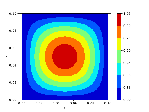
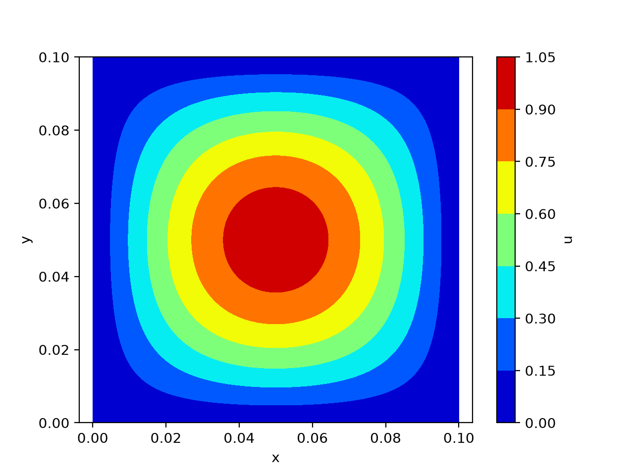
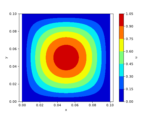
Temperature distribution at the initial moment of time.#
2. Mathematical statement of the problem#
The model of thermal conductivity in two-dimensional space is described by the equation (1).
where:
\( u(x,y,t) \) - temperature at the point with coordinates \( (x,y) \) at the moment of time \( t \);
\( \frac{\partial u}{\partial t} \) is a partial time derivative of temperature reflecting the rate of temperature change;
\( \frac{\partial^2 u}{\partial x^2} \) и \( \frac{\partial^2 u}{\partial y^2} \) – second partial derivatives on coordinates \( x \) and \( y \) respectively, which describe the diffusion distribution of temperature over space;
\( \alpha \) – thermal conductivity factor, which characterizes how quickly heat spreads in a material.
Often when writing partial equations, the symbols \(\partial \) are omitted for brevity. Then the variable by which the derivative is taken becomes the subscript. For example, the thermal conductivity equation in such notation would be:
To solve such equations, additional conditions are required to find a particular solution to the equation. At the initial moment of time \( t = 0 \), the temperature is specified analytically by the function:
At the boundary of domain \( \partial \Omega \), where \( \Omega = [0,1] imes [0,1] \), temperature is fixed and equal to zero:
For this problem formulation, the analytical solution can be obtained by the method of separation of variables (Fourier method). Suppose the solution is:
Substituting this representation into the original equation, after separating the variables and applying the boundary conditions (where \( X(0)=X(1)=0 \) and \( Y(0)=Y(1)=0 \)), we obtain the eigenfunctions for the spatial part:
The time function \( T(t) \) is determined from the ordinary differential equation:
from where
Thus, the complete analytic solution is written as follows:
This solution satisfies the initial condition and the zero boundary conditions. The evolution of the solution over time is as follows:
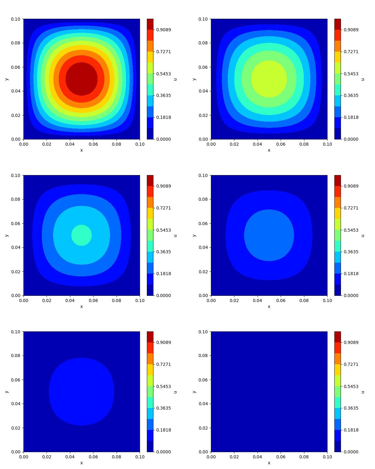
Evolution of the solution.#
3. PINN model description#
Physically-informed neural network (PINN) is an approach in which neural network is used to approximate the solution of a differential equation by integrating the residuals of the equation into the loss function.
In the case of the problem under consideration, a differential equation in domain \(\Omega \) with boundary and initial conditions is given. The analytical solution \( u(x,y,t) \) is approximated by a neural network \( \hat{u}(x,y,t; heta) \), where \( heta \) is the set of network parameters. In this case, the model takes spatial and temporal coordinates \( (x, y, t) \) as input, and returns an approximate temperature value \( u \).
Unlike most other tasks where neural networks are used, the PINN model does not have generalizability in the sense of solving a variety of problems. It only describes the solution of a specific problem in a given domain at any point in space and time. Thus, to find a value at time \( t_i \) we do not need to find values at times \( t_{i-1}, t_{i-2}, ... \), as would be needed, for example, when using finite differences or volumes - the method immediately returns a value for the submitted dataset. Moreover, the method is gridless, which means that the parameter value can be obtained at absolutely any point in the calculation domain. The PINN model can be considered as a kind of method for encrypting data about a process in a specific domain in the form of weights of a trained model.
Loss function in PINN usually consists of several terms:
Loss on equation
The problem is that network prediction satisfies the differential equation. To do this, calculate the remainder of the equation:
\[ f(x,y,t;\theta) = \hat{u}_t - \alpha \left( \hat{u}_{xx} + \hat{u}_{yy} \right). \]If there is no heat source in the domain, as in the problem posed, \( \lim\limits_{ heta o \hat{ heta}} f(x,y,t; heta) o 0\), where \(\hat{ heta} \) is the set of parameters at which the error on the equation is zero (absolute fit). The loss function for the remainder can be written as a mean square error:
\[ \mathcal{L}_{\text{PDE}} = \frac{1}{N_f} \sum_{i=1}^{N_f} \left| f(x_i, y_i, t_i;\theta) \right|^2. \]Loss at boundary conditions
For points belonging to the boundary \( \partial \Omega \), the model shall satisfy boundary conditions, for example, \( \hat{u}(x,y,t) = g(x,y,t) \). Loss of boundary conditions:
\[ \mathcal{L}_{\text{BC}} = \frac{1}{N_b} \sum_{i=1}^{N_b} \left| \hat{u}(x_i, y_i, t_i;\theta) - g(x_i, y_i, t_i) \right|^2. \]Loss on initial terms
If the initial conditions are \( \hat{u}(x,y,0) = h(x,y) \), then:
\[ \mathcal{L}_{\text{IC}} = \frac{1}{N_i} \sum_{i=1}^{N_i} \left| \hat{u}(x_i, y_i, 0;\theta) - h(x_i, y_i) \right|^2. \]
The general loss function is as follows:
where \( w_{ ext{PDE}} \), \( w_{ ext{BC}} \) and \( w_{ ext{IC}} \) are weighting factors that regulate the contribution of each term.
Thus, a display is generated, allowing to estimate the degree of correspondence of model predictions to the initial problem setting.
Then the model is trained, and the parameters \( heta \) are optimized using the selected optimization algorithm so as to minimize the overall loss function \( \mathcal{L}( heta) \).
Since the neural network models is trained using an error propagation method in which partial derivatives are calculated by parameters, the same tool can be used to find a derivative of predictions from the input data to check whether the predictions match the equation. Such a tool is automatic differentiation implemented in frameworks (for example, in PyTorch).
3.1. PINN method modifications#
To improve the convergence rate and overall solution accuracy for PINN models, the following refinements are applied:
Using non-standard activation features
Standard activation functions (e.g., Tanh or ReLU) may not be efficient enough to approximate complex functions with high-frequency components. Based on the fact that many solutions of equations are described in the form of harmonic functions (or series by them), it has been proposed to use the function sin as an activation function. An example of such a layer is:
where \( \omega_0 \) is a scale factor that amplifies high-frequency components. This modification allows the network to better approximate changes in the solution and provides faster convergence.
Hybrid optimizers
PINN training can face challenges due to the large dimension and nonlinearity of the problem. To solve this problem, a hybrid optimization approach is used, which combines the advantages of various optimizers:
Adam is a first-order gradient method, it quickly converges at the beginning of training due to adaptive step.
LBFGS is a quasi-Newtonian method, it is often used in the final stages to fine-tune parameters, which allows achieving higher accuracy due to the second order of information about the loss function.
The loss function is minimized first by the optimizer Adam[1], and then the model is further trained by the optimizer LBFGS[2] to increase the accuracy[3].
We apply these methods to solve the problem. However, note that there are other approaches, such as sequential or domain-specific learning, trainable activation functions, and others that are beyond the scope of this practical guide.
4. Building a PINN model#
Note
You can download the Jupyter laptop file if you want to quickly execute the code of this practice guide on your personal computer.
You can also download PINN file of the model and immediately apply it in a project on the REPEAT VISION platform using the block Approximation model.
To solve the problem, a neural network with a modified loss function will be used, as described in previous chapter. We will consider the model building taking into account the described modifications. For a simpler example, for a one-dimensional equation and without complications, you can read the corresponding tutorial.
Python language and framework PyTorch will be used to build the model, so basic knowledge of this language and skills with PyTorch are needed.
Important
Please note that to install a version of PyTorch that supports GPU operation and is compatible with your version of CUDA, you need to visit the official website.
First of all, we import the necessary libraries to create neural networks, build visualizations and then import into the ONNX format.
1import torch
2import torch.nn as nn
3import torch.optim as optim
4
5import numpy as np
6import matplotlib.pyplot as plt
7
8import onnx
9import json
To test the trained model, we obtain the analytical solution function. It will allow both to calculate the error according to \(L^2\) norm at a specific moment in time, and to perform a comparative analysis of the evolution of the solution obtained using PINN and the analytical solution.
 1def analytical_solution(x: np.ndarray,
 2                        y: np.ndarray,
 3                        t: np.ndarray,
 4                        bounds: dict,
 5                        alpha: float) -> np.ndarray:
 6    """
 7    Аналитическое решение
 8
 9    Параметры:
10        x: np.ndarray
11            Вектор координат x.
12        y: np.ndarray
13            Вектор координат y.
14        t: np.ndarray
15            Вектор координат t.
16        bounds: dict
17            Границы расчетной области.
18        alpha: float
19            Коэффициент температурапроводности материала.
20
21    Возвращает:
22        np.ndarray
23            Вектор значений температур, являющихся аналитическим решением.
24    """
25    u = (np.sin(np.pi * x/bounds['x']) * np.sin(np.pi * y/bounds['y'])
26         * np.exp(-2 * np.pi**2 * alpha * t/(bounds['x']*bounds['y'])))
27
28    return u
Rows 1-5. Definition of the function
analytical_solution, which computes the analytical solution of the heat equation in a two-dimensional domain.Row 25-26. Calculating the analytical solution according to the formula (5) taking into account the dimension:
\[ u(x, y, t) = \sin\left(\frac{\pi x}{L_x}\right) \sin\left(\frac{\pi y}{L_y}\right) \exp\left(-2 \pi^2 \alpha \frac{t}{L_x L_y}\right). \]where \( L_x \) и \( L_y \) are the dimensions of the region taken from
bounds['x']andbounds['y']respectively.
The function returns an array of temperature values based on coordinates, time, and material.
According to the arguments above, the use of the sine activation function helps to effectively describe various non-linear relationships, moreover, the analytical solution to the problem is also described using the sine. Using the conclusions from the article[4] and using as a basis the code presented by the authors, we implement a linear layer with a sinusoidal activation function. To achieve convergence, it is necessary to take into account the characteristics of initializing the layer weights and select some hyperparameters, the theoretical justification of this process is presented in the original article.
Let us create a linear layer class with a sinusoidal activation function, as a refinement of the linear layer taking into account all the mentioned features.
 1class SinLayer(torch.nn.Module):
 2    """
 3    Слой нейронной сети с синусоидальной функцией активации.
 4
 5    Параметры:
 6        in_features: int
 7            Количество входных признаков.
 8        out_features: int
 9            Количество выходных признаков.
10        bias: bool
11            Использовать ли смещение в линейном слое.
12        is_first: bool
13            Является ли слой первым в сети.
14        omega_0: float
15            Частота для функции синуса.
16    """
17    def __init__(self,
18                 input: float,
19                 output: float,
20                 bias: bool=True,
21                 is_first: bool=False,
22                 omega_0: float=30):
23        super().__init__()
24        self.omega_0 = omega_0
25        self.is_first = is_first
26        self.in_features = input
27        self.linear = torch.nn.Linear(input, output, bias=bias)
28        self.init_weights()
29
30    def init_weights(self):
31        """
32        Инициализация весов линейного слоя.
33        """
34        with torch.no_grad():
35            if self.is_first:
36                self.linear.weight.uniform_(-1 / self.in_features,
37                                            1 / self.in_features)
38            else:
39                self.linear.weight.uniform_(-np.sqrt(6 / self.in_features)
40                                            / self.omega_0,
41                                            np.sqrt(6 / self.in_features)
42                                            / self.omega_0)
43
44    def forward(self, input):
45        """
46        Прямой проход через слой.
47
48        Параметры:
49            input: torch.Tensor
50                Входной тензор.
51
52        Возвращает:
53            torch.Tensor
54                Результат применения синусоидальной функции активации.
55        """
56        return torch.sin(self.omega_0 * self.linear(input))
Row 1. Definition of the class
SinLayerwhich is a layer of a neural network with a sinusoidal activation function.Rows 17-22. Definition of a constructor for the
__init__class that accepts layer parameters.Rows 23-27. Initialization of parameters
omega_0,is_first,in_featuresand creation of a linear layer (torch.nn.Linear).Row 28. Call for the
init_weights()method, which sets the initial values of the weights.Row 30. Definition of the
init_weights()method that sets the initial values of the linear layer weights.Rows 35-37. If the layer is first (
is_first = True), the weights are initialized uniformly in the range \( [\frac{-1}{ ext{in}\_ ext{features}}, \frac{1}{ ext{in}\_ ext{features}}] \).Row 38-42. Otherwise, the weights are initialized in the range \( \left[-\frac{\sqrt{6 / ext{in}\text{features}}}{\omega_0}, \frac{\sqrt{6 / ext{in}\text{features}}}{\omega_0} ight] \), which improves convergence when training the network.
Row 44. Definition of a
forward()method that performs a forward pass through a layer.Row 56. Applying a linear layer to the input data, multiplying the result by the
omega_0frequency and passing it to thetorch.sin()function that implements sinusoidal activation.
Such a layer is used in neural network architectures such as SIREN (Sinusoidal Representation Networks) and allows efficient approximation of a wide range of dependency frequencies in data of different types.
Now let us create a neural network architecture. The SinPINN class is a fully connected network consisting of several linear layers with a sinusoidal activation function(instances of the SinLayer class). The model takes the coordinates \( (x, y) \) and time \( t \) at the input, and outputs the predicted temperature \( u \) points, with coordinates \( (x, y) \) at the moment of time \( t \).
 1class SinPINN(nn.Module):
 2    """
 3    Физически-информированная нейронная сеть (PINN) с функцией активации синус.
 4
 5    Параметры:
 6        layers: nn.ModuleList
 7            Список слоёв нейронной сети.
 8    """
 9    def __init__(self,
10                 layers: list):
11        super().__init__()
12        self.layers = nn.ModuleList()
13        for i in range(len(layers) - 1):
14            if i == 0:
15                self.layers.append(SinLayer(layers[i],
16                                            layers[i+1], is_first=True))
17            elif i == len(layers) - 2:
18                self.layers.append(nn.Linear(layers[i],
19                                             layers[i+1],))
20            else:
21                self.layers.append(SinLayer(layers[i],
22                                            layers[i+1], is_first=False))
23
24    def forward(self,
25                x: torch.Tensor,
26                y: torch.Tensor,
27                t: torch.Tensor) -> torch.Tensor:
28        """
29        Прямой проход через сеть.
30
31        Параметры:
32            x: torch.Tensor
33                Тензор координат x.
34            y: torch.Tensor
35                Тензор координат y.
36            t: torch.Tensor
37                Тензор время t.
38
39        Возвращает:
40            torch.Tensor
41                Выход сети.
42        """
43        inputs = torch.cat([x.reshape(-1, 1),
44                            y.reshape(-1, 1),
45                            t.reshape(-1, 1)], dim=1)
46        for layer in self.layers:
47            inputs = layer(inputs)
48        return inputs
Row 1: Declaration of the
SinPINNclass, which inherits functionality from thenn.Modulebase class of thePyTorchlibrary. This provides the ability to use all built-in mechanisms to build and train neural networks.Row 9: Declaring a class constructor that accepts
layers— a list that defines the number of neurons for each layer of the network.Row 11: Calling the base class constructor
nn.Moduleto correctly initialize all the internalPyTorchmechanisms required to work with neural networks.Row 12: Initialize the
ModuleListobject to store neural network layers. Using ofModuleListallows to automatically register the parameters of all added layers.Row 13–22: Cycle on the indexes of the
layerslist creating the layers of the neural network. Separately, it is checked whether the layer is the first layer in the network. If this condition is fulfilled, aSinLayerwith the flagis_first=Trueis created. If the last layer is encountered, a regularLinearlayer without a sinusoidal activation function is created. In other cases,SinLayeris created withis_first=False.Row 24: Declaration of the ‘forward’ method, which specifies the order in which input data passes through the network. This method takes the tensors
x,yandtas input and returns the model prediction (temperature).Rows 43-45: Merging the input data (coordinates
x,yand timet) into one tensor. The data is converted from vectors into 2D tensors of dimension(-1, 1)and concatenated along thedim=1axis, that is, along the column axis. The result is a matrix, in the rows of which certain states of the system \( x_i, y_i, t_i \) are recorded.
Note
x.reshape(-1, 1):
-1 indicates that PyTorch will automatically substitute the number of rows equal to the number of elements in x.
1 specifies the number of columns to convert the one-dimensional tensor (N,) into a two-dimensional tensor (N,1).
Row 46–47: Loop to pass data through all layers.
Attention
Note that the activation function in this case is integrated into layers.
Row 48: Return an output tensor
inputscontaining the predicted values obtained by forward passing through the entire network.
4.1. Definition of loss function.#
The loss function includes three components:
Initial loss — comparison of predicted temperature at time \( t=0 \).
Boundary condition loss — compares the predicted temperature at points \( (x, y) \in \partial \Omega \), where \( \Omega = [0,L] imes [0,L] \).
Loss for equation — a misalignment calculated by differential equation \( u_t - \alpha (u_{xx} + u_{yy}) = 0 \).
First, consider the loss component for the equation and write a function to calculate it.
 1def pde_residual(model: SinPINN,
 2                 x: torch.Tensor,
 3                 y: torch.Tensor,
 4                 t: torch.Tensor,
 5                 alpha: float):
 6    """
 7    Вычисляет остаток по уравнению теплопроводности для модели PINN.
 8    Вид уравнения:
 9        u_t - alpha * (u_xx + u_yy) = 0
10
11    Параметры:
12        model: torch.nn.Module
13            Модель, вычисляющая u(x, y, t).
14        x: torch.Tensor
15            Тензор координаты x.
16        y: torch.Tensor
17            Тензор координаты y.
18        t: torch.Tensor
19            Тензор времени t.
20        alpha: float
21            Коэффициент теплопроводности.
22
23    Возвращает:
24        torch.Tensor
25            Остаток уравнения f = u_t - alpha*(u_xx + u_yy).
26    """
27    u = model(x, y, t)
28
29    u_x, u_y, u_t = torch.autograd.grad(u, [x, y, t],
30                                        grad_outputs=torch.ones_like(u),
31                                        create_graph=True)
32
33    u_xx = torch.autograd.grad(u_x, x, grad_outputs=torch.ones_like(u_x),
34                               create_graph=True)[0]
35    u_yy = torch.autograd.grad(u_y, y, grad_outputs=torch.ones_like(u_y),
36                               create_graph=True)[0]
37
38    f = u_t - alpha * (u_xx + u_yy)
39    return f
Row 1. Declaration of the function
pde_residual, which takes as arguments a model, tensors of points by coordinates and time to calculate the residuals (inconsistency) of the equation. The function returns the total value of the loss function on the equation.Row 27. Calculation of the value of the model output \( u(x, y, t) \).
Row 29-31. Calculation of the first derivatives of \( u_x, u_y, u_t \) using the autodifferentiation function
torch.autograd.grad. The parametergrad_outputs=torch.ones_like(u)indicates that the derivative is calculated for each element of the tensoru. Thecreate_graph=Trueflag allows to build a computational graph for further differentiation, which is necessary to calculate the second derivative.Row 33-35. Calculation of the second derivatives of \( u_{xx} \) and \( u_{yy} \) on
xandyrespectively, usingtorch.autograd.gradin the same way.Row 38. Calculation of the remainder of the thermal conductivity equation. If the model predictions satisfy the physical equation (2), \( f = u_t - \alpha (u_{xx} + u_{yyy})\) shall tend to zero.
Row 39. Return of the result
f, which will then be used to train PINN.
4.2. Data preparation and model training#
To verify that the problem equations fulfill the model predictions, we need to create a set of points on which to read the loss function. Since the problem is formulated by three equations (heat transfer equation, initial and boundary conditions), we will create sets of collocation points for each of the equations, respectively.
 1def generate_pde_points(n: int,
 2                        bounds: dict,
 3                        device: torch.device):
 4    """
 5    Генерирует точки коллокации для уравнения PDE.
 6
 7    Параметры:
 8        n: int
 9            Число точек коллокации.
10        bounds: dict
11            Границы области.
12        device: torch.device
13            Устройство (CPU или GPU).
14
15    Возвращает:
16        Tuple[torch.Tensor, torch.Tensor, torch.Tensor]
17            Тензоры x, y, t с requires_grad=True.
18    """
19    x = (bounds['x'] * torch.rand(n, 1, device=device)).requires_grad_()
20    y = (bounds['y'] * torch.rand(n, 1, device=device)).requires_grad_()
21    t = (bounds['t'] * torch.rand(n, 1, device=device)).requires_grad_()
22    return x, y, t
Row 1. Declaration of the function
generate_pde_points, which generates collocation points for calculating the residuals of a solution to a differential equation.Row 19-21. Generation of random values for coordinates
x,y,twithin the specifiedboundsin two steps:Creates random values from 0 to 1 using
torch.rand(n, 1, device=device).Multiplying by
bounds['x'],bounds['y'],bounds['t']scales points to the specified boundaries of the calculated domain. Callingrequires_grad_()method allows to calculate gradients with respect to these variables.
Row 22. Return of generated tensors
x,y,t.
 1def generate_initial_condition(n: int,
 2                               bounds: dict,
 3                               device: torch.device):
 4    """
 5    Генерирует точки для начального условия.
 6
 7    Параметры:
 8        n: int
 9            Число точек начального условия.
10        bounds: dict
11            Границы расчетной области.
12        device: torch.device
13            Устройство (CPU или GPU).
14
15    Возвращает:
16        Tuple[torch.Tensor, torch.Tensor, torch.Tensor, torch.Tensor]:
17            Тензоры x, y, t, u,
18            где t — нулевой тензор, а u = sin(pi * x/L) * sin(pi * y/L).
19    """
20    x = bounds['x'] * torch.rand(n, 1, device=device)
21    y = bounds['y'] * torch.rand(n, 1, device=device)
22    t = torch.zeros_like(x, device=device)
23    u = torch.sin(np.pi * x/bounds['x']) * torch.sin(np.pi * y/bounds['y'])
24    return x, y, t, u
Row 1. Declaring a
generate_initial_conditionfunction that creates points to check the initial condition.Rows 20-21. Generating random values for
xandywithin boundaries, similar to the method in thegenerate_pde_pointsfunction.Row 22. Setting
t = 0since the initial conditions are set at time \( t=0\).Row 23. Calculating
ubased on the initial condition (3) \( u = \sin(\pi x/L) \sin(\pi y/L) \).Row 24. Return of generated tensors
x,y,t,u.
 1def generate_boundary_conditions(n: int,
 2                                 bounds: dict,
 3                                 device: torch.device):
 4    """
 5    Генерирует точки граничных условий.
 6
 7    Параметры:
 8        n_b: int
 9            Число точек для граничных условий.
10        bounds: dict
11            Границы области, например, {'x': 1.0, 'y': 1.0, 't': 1.0}.
12        device: torch.device
13            Устройство (CPU или GPU).
14
15    Возвращает:
16        Tuple[torch.Tensor, torch.Tensor, torch.Tensor, torch.Tensor]:
17            x_b, y_b, t_b, u_b, где u_b = 0.
18    """
19    x = bounds['x'] * torch.rand(n, 1, device=device)
20    y = bounds['y'] * torch.rand(n, 1, device=device)
21    t = bounds['t'] * torch.rand(n, 1, device=device)
22
23    border_selector = torch.randint(0, 4, (n, 1), device=device)
24    x[border_selector == 0] = 0.0 # Left bound
25    x[border_selector == 1] = bounds['x'] # Right bound
26    y[border_selector == 2] = 0.0 # Bottom bound
27    y[border_selector == 3] = bounds['y'] # Upper bound
28
29    u_b = torch.zeros_like(t, device=device)
30    return x, y, t, u_b
Row 1. Declaring a
generate_boundary_conditionsfunction that creates points to check boundary conditions.Rows 19-21. Generation of random points
x,y,twithin the boundaries, similar to the method in the functiongenerate_pde_points.Row 23. Creating a
border_selectorthat randomly selects boundary points.Rows 24-27. Assigning boundary coordinate values
x=0,x=L,y=0,y=Ldepending onborder_selector.Row 29. Setting the zero boundary condition
u_b = 0according to the condition (4).Row 30. Return of generated tensors
x,y,t,u_b.
To achieve reproducibility of results, fix random generation. To speed up subsequent calculations, we will determine the available device (GPU, if available, or CPU).
We declare the parameters of the problem, such as the number of collocation points of different types, the boundaries of the computational domain in space and time, and the temperature conductivity factor
 1torch.manual_seed(42)
 2np.random.seed(42)
 3
 4device = torch.device("cuda" if torch.cuda.is_available() else "cpu")
 5
 6N_F, N_B, N_I = 10000, 5000, 2000
 7BOUNDS = {'x': 0.1, 'y': 0.1, 't': 12.0}
 8ALPHA = 1.12 * 1e-4
 9
10model = SinPINN([3, 64, 1]).to(device)
11mse_loss = nn.MSELoss()
12optimizer = optim.Adam(model.parameters(), lr=1e-3)
13
14x_f, y_f, t_f = generate_pde_points(N_F, BOUNDS, device)
15x_i, y_i, t_i, u_i = generate_initial_condition(N_I, BOUNDS, device)
16x_b, y_b, t_b, u_b = generate_boundary_conditions(N_B, BOUNDS, device)
17
18w_pde, w_bc, w_ic = 10.0, 1.0, 1.0
Row 1. Setting
torch.manual_seed(42)to ensure experiment reproducibility when using PyTorch.Row 2. Setting
np.random.seed(42)to ensure reproducibility for the NumPy library.Row 4. Specifying the computing device
device(GPU, if available, or CPU).Row 6. Determination of the number of collocation points for the equation (
N_F), for the boundary conditions (N_B), for the initial condition (N_I).Row 7. Defining the boundaries of the computational domain along the x-axis, along the y-axis, and the maximum value of the simulation time in the form of the
BOUNDSdictionary.Row 8. Defining of thermal conductivity factor corresponding to copper
ALPHA = 1.12 * 1e-4.Row 10. Creating a
SinPINNmodel with one hidden layer of 64 neurons and transfer the model to thedevice.Row 11. Defining the loss function
mse_lossthat uses the standard error (MSE).Row 12. Defining an
Adamoptimizer to update model parameters.Rows 14-16. Generation of training data (collocation points) for the corresponding parts of the task setting.
Row 18. Formal definition of weights for different parts of the loss function. They can be adjusted for better convergence or for specific values.
Let us move on to model training. The main training cycle takes place during a given number of eras, where at each era:
Zero gradients.
The components of the loss function are calculated.
The error is propagated back.
Model parameters are updated.
The value history of the loss function components is saved.
Periodically output the loss value to monitor the training process.
 1epochs = 20000
 2
 3loss_history = {'pde': [],
 4                'ic': [],
 5                'bc': []}
 6
 7for epoch in range(epochs+1):
 8    optimizer.zero_grad()
 9
10    u_pred_i = model(x_i, y_i, t_i)
11    loss_ic = mse_loss(u_pred_i, u_i)
12
13    u_pred_b = model(x_b, y_b, t_b)
14    loss_bc = mse_loss(u_pred_b, u_b)
15
16    loss_pde = mse_loss(pde_residual(model, x_f, y_f, t_f, ALPHA),
17                        torch.zeros_like(x_f))
18
19    loss = w_ic * loss_ic + w_bc * loss_bc + w_pde * loss_pde
20
21    loss.backward()
22    optimizer.step()
23
24    loss_history['ic'].append(loss_ic.item())
25    loss_history['bc'].append(loss_bc.item())
26    loss_history['pde'].append(loss_pde.item())
27
28    if epoch % 1000 == 0:
29        print(f"Epoch {epoch}, Loss: {loss.item():.3e}, "
30              f"IC: {loss_ic.item():.3e}, "
31              f"BC: {loss_bc.item():.3e}, "
32              f"PDE: {loss_pde.item():.3e}")
Row 1. The number of epochs is set, which determines the number of iterations of model training.
Rows 3-5. A dictionary
loss_historyis created to store the values of the loss function components.Rows 7-30. The basic cycle of model training. Each of its epochs contains the following occurences:
Zeroing optimizer gradients.
Calculation of the error for the initial condition. The model predicts
uvalues for the initial condition points, then calculates the mean squared error from these relative to the trueuvalues.Similarly, an error is calculated for boundary conditions.
The calculation of the equation error is performed in the above-described
pde_residualfunction, to which the corresponding input parameters are transmitted, and the output tensor is compared with zero.All components of the loss function are added to the corresponding weights.
Model parameter gradients are calculated taking into account all components of losses.
The optimization step updates the model parameters.
Then the values of the loss function components are saved and output periodically.
To visually assess the quality of the learning process, we can visualize the values of the components of the loss function from epochs on a logarithmic scale.
 1def plot_loss_history(loss_history: dict,
 2                      step: int=200):
 3    """
 4    Функция для построения графика функции потерь.
 5
 6    Параметры:
 7        loss_history : dict
 8            Словарь, содержащий данные для потерь.
 9        step : int, optional
10            Шаг выборки данных для отображения, по умолчанию 100.
11    """
12    epochs = range(0, len(loss_history['pde']), step)
13
14    plt.plot(epochs, loss_history['pde'][::step], label='PDE Loss')
15    plt.plot(epochs, loss_history['bc'][::step], label='BC Loss')
16    plt.plot(epochs, loss_history['ic'][::step], label='IC Loss')
17
18    plt.yscale('log')
19    plt.xlabel('Epoch')
20    plt.ylabel('Loss')
21    plt.grid()
22    plt.legend()
23    plt.show()
Rows 1-2. Declaration of
plot_loss_historyfunction to plot the loss function.Row 12. Defines a list of
epochsthat contains epoch numbers, instepincrements. It is necessary for correct display of the epoch number on the \(x\) axis.Rows 14-16. The graphs are plotted for each of the loss components, with values taken in
stepincrements for greater smoothness.
Let us call this function by sending it the training history loss_history.
1plot_loss_history(loss_history)
A graph of the following form will be plotted:
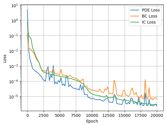
Loss function graph.#
In addition to Adam optimization, the quasi-Newtonian method LBFGS is often used. It is computationally more complicated, but is well suited for quadratic loss functions, which we use, allowing to find the minimum in a few iterations. However, LBFGS tends to fall within local lows on descent, while Adam has no such drawback. For these reasons, they are used together and exactly in the sequence indicated.
Due to slightly different interface of interaction in the implementation of the LBFGS method in the PyTorch library from other optimizers, it is necessary to declare an auxiliary function closure, which will be called when the optimizer is running.
 1def closure():
 2    """
 3    Вспомогательная функция для оптимизатора LBFGS.
 4    """
 5    optimizer_lbfgs.zero_grad()
 6
 7    loss_ic = mse_loss(model(x_i, y_i, t_i), u_i)
 8
 9    loss_bc = mse_loss(model(x_b, y_b, t_b), u_b)
10
11    loss_pde = mse_loss(pde_residual(model, x_f, y_f, t_f, ALPHA),
12                           torch.zeros_like(x_f))
13
14    loss = w_ic * loss_ic + w_bc * loss_bc + w_pde * loss_pde
15
16    loss.backward()
17
18    return loss
19
20optimizer_lbfgs = optim.LBFGS(model.parameters(), lr=1.0,
21                              max_iter=500, history_size=50)
22optimizer_lbfgs.step(closure)
Row 1-18. A
closurefunction is created that will be used for optimization using theLBFGSmethod. The following actions take place therein:Zeroing optimizer gradients.
Calculation of the loss function from initial and boundary conditions and from the equation using the previously defined
pde_residualfunction.The resulting components are summed with the weights, yielding the final
lossloss function.The gradients of the model are computed by calling
loss.backward().
Rows 20-21. An optimizer object
LBFGSis created, into which the model parameters, the training rate, the maximum number of iterations and the size of the optimization history are transmitted.Row 22. An optimization step is performed using the
closurefunction, updating the model parameters to minimize the loss function.
Thus, we obtained a trained model to solve the given problem
5. Exporting a model to ONNX format#
After training, the model is converted to double precision mode using the double() method. Then, using the input tensor template, the model is exported to ONNX format. In this case, the names of the input and output parameters are specified for correct integration.
 1model.double()
 2
 3# Создание тестового входного тензора (x, y, t)
 4x_temp = torch.randn(1, 1, device=device, dtype=torch.float64) * BOUNDS['x']
 5y_temp = torch.randn(1, 1, device=device, dtype=torch.float64) * BOUNDS['y']
 6t_temp = torch.randn(1, 1, device=device, dtype=torch.float64) * BOUNDS['t']
 7
 8input_names = ['x', 'y', 't']
 9output_names = ['u']
10
11torch.onnx.export(model,
12                  (x_temp, y_temp, t_temp),
13                  "pinn_heat2d.onnx",
14                  opset_version=12,
15                  input_names=input_names,
16                  output_names=output_names)
Row 1. Set model to double precision
float64mode. This is important for accurate calculations when working with partial differential equations.Rows 4-6. Creating of test input tensors
x_temp, y_temp, t_tempwith random values scaled by BOUNDS.Rows 8-9. Defining the names of the input \((x, y, t)\) and output \((u)\) parameters of the model.
Rows 11-16. Export the model to ONNX format with the following parameters:
model — object of class
SinPINN.(x_temp, y_temp, t_temp) — tuple of input tensors.
“pinn_heat2d.onnx” — the output file name.
opset_version=12 — ONNX API version.
input_names and output_names — the names of the input and output parameters.
Additionally, for integration into REPEAT VISION it is necessary to add metadata about the boundaries of the calculation area.
:caption: Добавление метаданных в файл
:lineno-start: 1
# Загрузка экспортированной модели ONNX
onnx_model = onnx.load("pinn_heat2d.onnx")

# Создание словаря метаданных с границами параметров x, y, t
metadata_dict = {
    "x": f"{BOUNDS['x']}",
    "y": f"{BOUNDS['y']}",
    "t": f"{BOUNDS['t']}"
}
metadata_json = json.dumps(metadata_dict)

metadata_prop = onnx.StringStringEntryProto()
metadata_prop.key = "bounds"
metadata_prop.value = metadata_json

# Добавление метаданных и сохранение обновленной модели
onnx_model.metadata_props.append(metadata_prop)
onnx.save(onnx_model, "pinn_heat2d.onnx")
Row 2. Loading a previously exported ONNX model.
Rows 5-9. Creating a dictionary metadata_dict containing the bounds of the input parameters.
Row 10. Converting the dictionary to JSON format.
Rows 12-14. Creating a StringStringEntryProto object to store key-value pairs.
Row 17. Adding metadata to the ONNX model.
Row 18. Saving the updated model to file “pinn_heat2d.onnx”.
6. Creating a project on the REPEAT VISION platform#
To begin with, a new project in REPEAT VISION should be created and a name, such as 2D thermal conductivity with PINN should be given. After creating the project, set the Simulation Time parameter to 12 [s] according to what was used earlier in training the model.
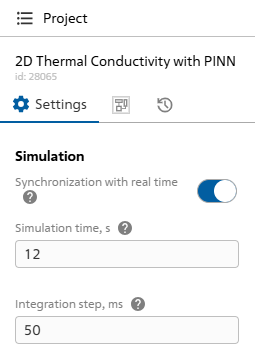
Fig. 1 Simulation time#
6.1. Importing a ONNX format model#
First of all, import the trained model saved in ONNX format into the REPEAT VISION project. To do this, open the library External models and move the block Approximation model to the workspace.
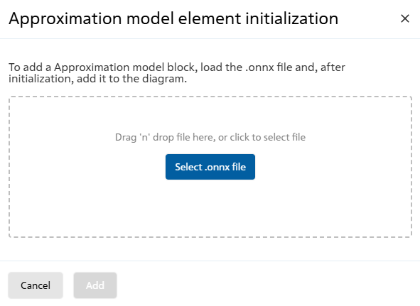
Fig. 2 Initialization of the Approximation model block#
Select the previously created model file in the explorer window. The model will be automatically loaded and initialized.
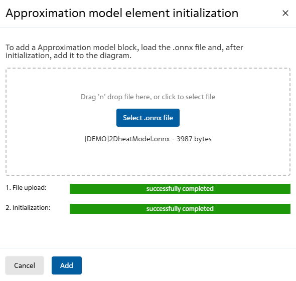
Fig. 3 Model initialization completed#
Important
Note that after importing the model, the number of input and output ports was determined automatically. It shall match those specified when exporting the model to ONNX. If this is not the case, an error was made as a result of the export.
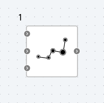
Fig. 4 Input and output ports#
Any values from the modeling area, either in the form of constants or any dependencies, can be supplied as coordinates. Let’s create coordinate blocks, for simplicity we’ll designate them with constant values and place them in the center of the calculation area - the point \((0.05, 0.05)\). To do this, add two Constant blocks from the Automation and connect them to the corresponding inputs of the approximation block.
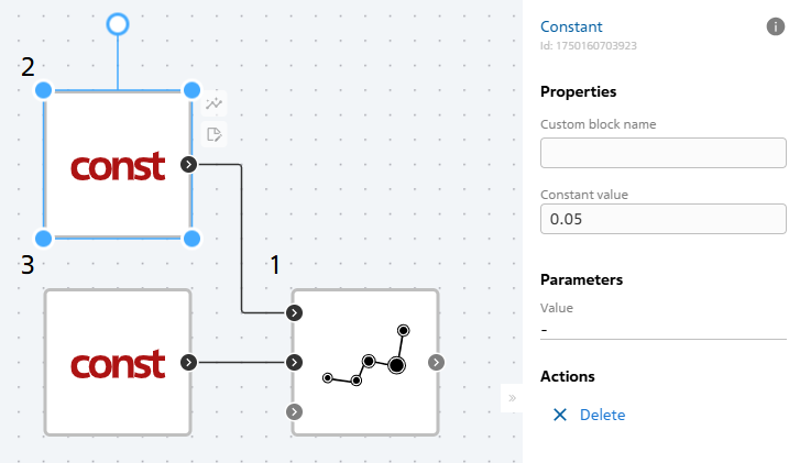
Fig. 5 Adding Constant blocks#
The simulation time value can be transmitted as time using the Simulation time block from the Simulation library. Let’s connect the corresponding block and connect it to the last input of the approximation block.
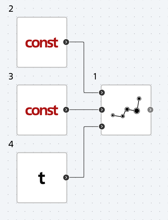
Fig. 6 Adding Simulation time block#
To get the output value of the model, let’s use the Outport block from the {bdg-muted}`External models library.
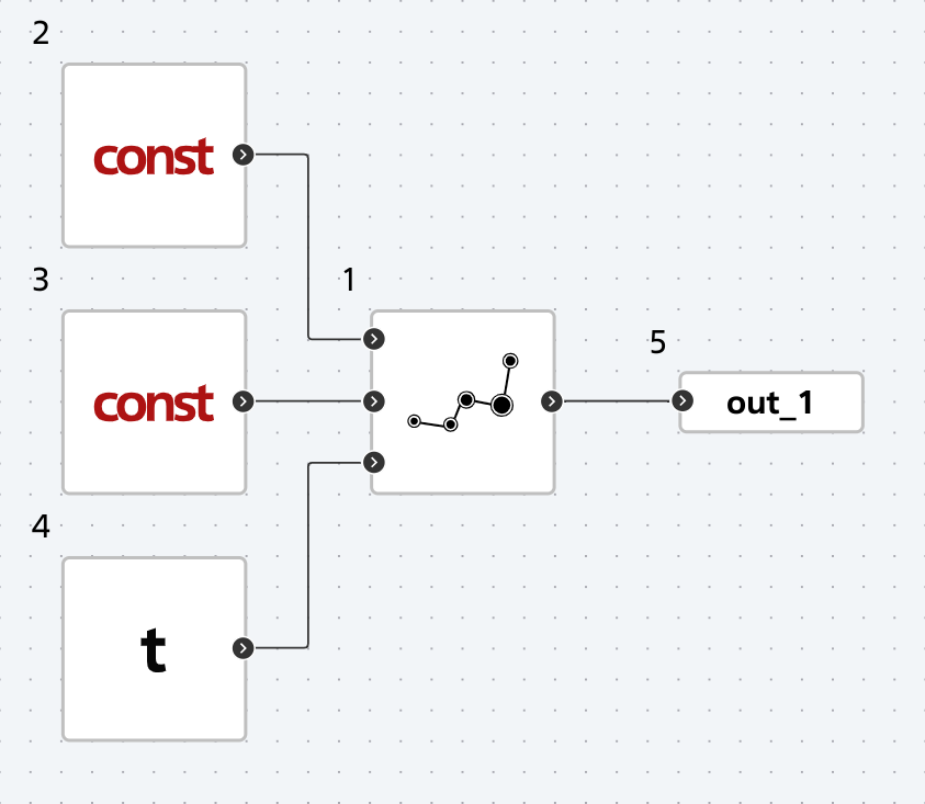
Fig. 7 Adding Outport block#
Let us add visualization of the output port to plot the dependence of the coordinate on time.
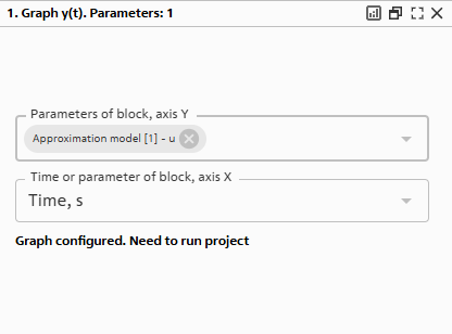
Fig. 8 Creating a graph#
7. Start calculation#
Run the calculation with the “Run Simulation!” button  . The calculation shall be successfully completed with the following message:
Modeling stopped on the solver side due to modeling time limit exceeded.
The visualization tab should plot the temperature versus time graph for the center point of the body.
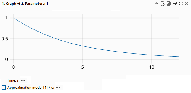
Fig. 9 Graph of results calculation#
8. Summary#
As part of this practical guide, you:
Gained a more detailed understanding of using neural networks to solve physical problems.
Applied current techniques to improve the convergence of PINN models in the form of a sinusoidal activation function and the use of several optimizers.
Improved skills in creating and training neural network models using
PyTorch.Mastered the export to
ONNXformat and subsequent integration into the project on the REPEAT VISION platform.Learned how to add bivariate dependency accounting to the REPEAT VISION solver.