A simple machine learning model of thermal conductivity

This practical guide presents the steps for implementing a simple Machine learning model designed to approximate the steady-state process of heat transfer by thermal conductivity in the wall of a product part, and also presents a method for using the ML model on the REPEAT VISION platform.

Note

If you do not have basic knowledge of using the REPEAT VISION Heat Exchange library, please read the introductory tutorial before continuing with this tutorial.

1.  Statement of the problem of heat transfer by thermal conductivity in the wall of a product part

To focus on the process of creating a machine learning model, it is necessary to prepare a simple problem of calculating the heat flow in the wall of a product part with a given thermal conductivity. The task will be based on the introductory tutorial of the Heat exchange library of the REPEAT VISION platform.

A project diagram with a name such as Thermal conductivity in a wall for calculating the heat flow in the wall of a product part is shown in the figure below and is described by the equation of block №1 Conductive heat transfer.

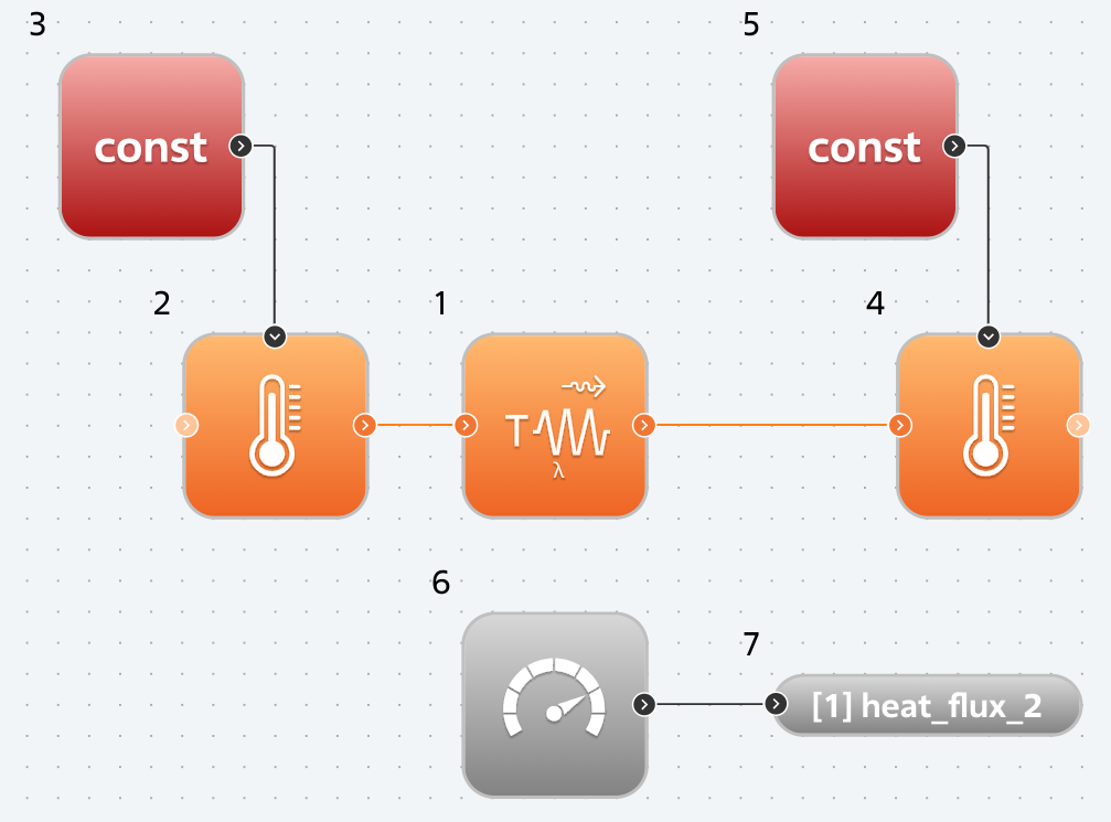
Model for calculating heat flow in the wall of a product part.

The project shown above allows one to investigate the change in the heat flux resulting from the calculation as the parameters given in the table below change.

Parameter	Parameter type	Global variable name	Applies to block
Internal wall temperature	Boundary condition \([^{\circ}C]\)	TEMPERATURE_1	block №3
External wall temperature	Boundary condition \([^{\circ}C]\)	TEMPERATURE_2	block №5

block №1 Conductive heat transfer has the following settings:

Property	Meaning
Wall geometry type	Plane
Surface area \([m^2]\)	3
Wall thickness, \([m]\)	0.005
Conductivity type	Constant
Thermal conductivity, \([W/m^{\circ}C]\)	1.4

The heat flux calculation result \([W]\) is passed from block №6 Meter to block №7 Outport with the user name heat_flux_2.

For this stationary problem statement, it will be sufficient to use the following project settings:

Simulation time \([s]\)	Integration step \([ms]\)	Sampling step \([ms]\)
0.1	50	50

1.1.  Requirements for formulating a problem for preparing a machine learning model

Taking into account the requirements for the machine learning model for further integration into the REPEAT VISION platform for interaction with the Heat exchange library blocks, the following describes the case of formulating the problem, in which the heat flux heat_flux_2 is positively directed from block №2 with the boundary condition of temperature TEMPERATURE_1 to block №4 with the boundary condition of temperature TEMPERATURE_2. This case is separately described in the help of the Approximation model (Heat exchange) block and looks like this.

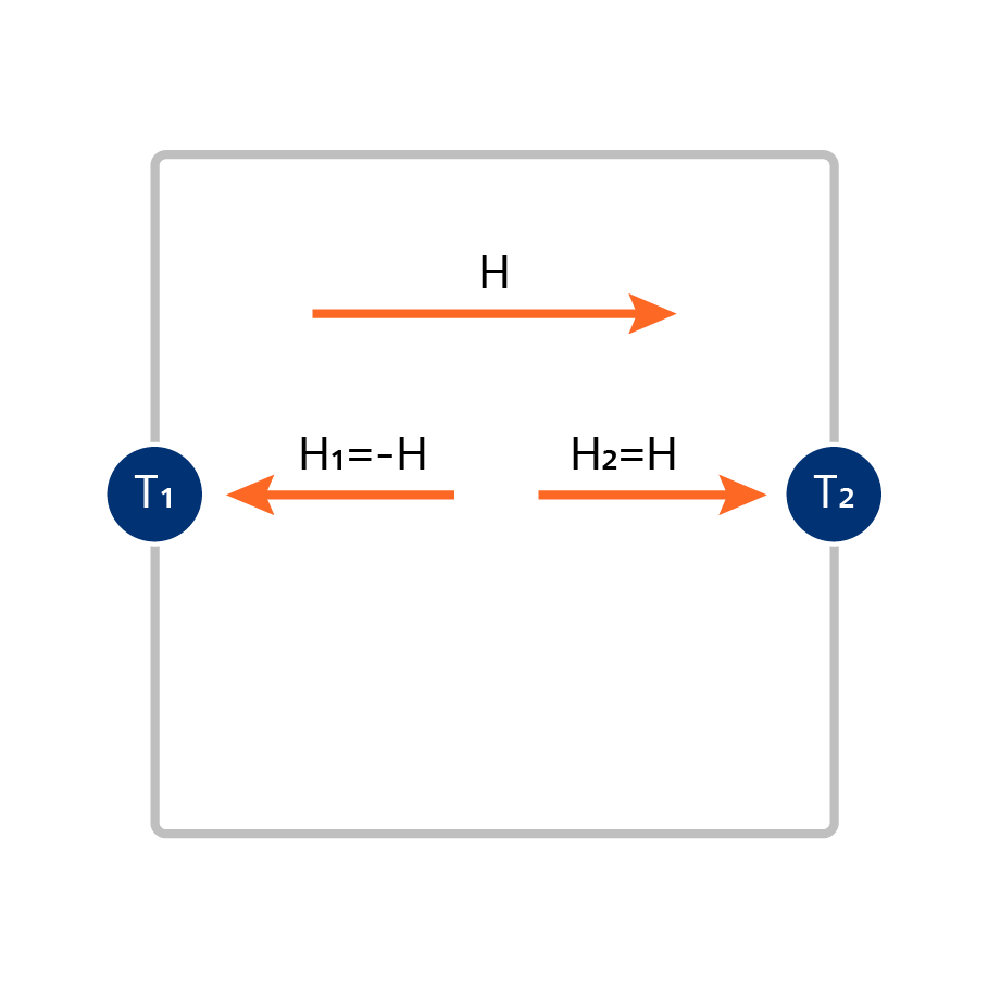
Calculation of heat flow from node 1 to node 2 of an approximation model with two nodes.

The diagram above uses the following notations.

Designations	Description
T1	Model node with temperature boundary condition TEMPERATURE_1
T2	Model node with temperature boundary condition TEMPERATURE_2
H →	Positive direction of heat flow of the heat_flux_2 model

When preparing heat flow calculation data for parametric studies, it is necessary to create an additional flux heat_flux_1 equal to the negative value of heat_flux_2 in accordance with the diagram given above.

2.  Preparing for work

Note

You can download the Jupyter notebook file and the ML model training data if you want to quickly complete this tutorial on your personal computer.

You can also download the ML model file and immediately use it in a project on the REPEAT VISION platform using the Approximation model (Heat exchange) block.

All subsequent data preparation and ML model creation must be performed locally due to the use of PyTorch for machine learning. It is recommended that this work be performed in Jupyter.

Before you begin, you need to install the Python repeat package, which is necessary for interacting with the REPEAT VISION platform, as well as install packages for working with data and creating ML models.

You need to run the following commands in the command line of your computer and continue working in the Jupyter notebook.

Bash

mkdir ml_heat_transfer
cd ml_heat_transfer
python -m venv repeat_ml.
source repeat_ml/bin/activate
python -m pip install repeat torch scikit-learn pandas onnx matplotlib tqdm jupyterlab ipywidgets

jupyter lab

PowerShell

mkdir ml_heat_transfer
cd ml_heat_transfer
python -m venv repeat_ml.
repeat_ml\Scripts\Activate.ps1
python -m pip install repeat torch scikit-learn pandas onnx matplotlib tqdm jupyterlab ipywidgets

jupyter lab

See also

For more information on using Python on your local machine to interact with the REPEAT VISION platform, please see our tutorials:

1. Using Python in CPython classic implementation

2. Preparing for work on approximating the solution of the differential equation of oscillations using PINN

In the first cell of your notebook, import the Python packages needed to prepare the data and process the calculation results, as well as the Python package repeat with the parametric studies module.

import numpy as np
import pandas as pd
import torch
import torch.nn as nn
import torch.optim as optim
from sklearn.model_selection import train_test_split
from tqdm.notebook import tqdm
import matplotlib.pyplot as plt
import repeat as rp
import repeat.parametric_study as ps

3.  Data preparation

To subsequently create a machine learning model, it is necessary to prepare a dataset that includes:

1. Temperature boundary conditions of the previously created heat conduction model;

2. Results of heat flow calculations for each calculation case.

To prepare the required data set, algorithms for performing parametric studies models for calculating heat flows in the wall of a product part will be required.

See also

A detailed practical guide to performing parametric studies is given in the relevant section of the REPEAT VISION documentation.

Below is a brief description of the main steps for calculating a set of heat flows in the wall of a product part on the temperature parameters grid of the model.

First, you need to set up a connection to the REPEAT VISION platform and select a model to perform parametric studies.

user = rp.User(
  "enter a unique API key from REPEAT VISION user cabinet instead of this comment"
  )
app = rp.Application(user)
# enter a project ID from REPEAT VISION application instead of 12345
project = 12345
t_interval = rp.TimeInterval(start = 50, end = 100)
model = app.get_exploration_model(project, t_interval)
print(model, model.existing_variables, sep = "\n")

For the algorithm for preparing a grid of temperature parameter values, in the next cell, create a dictionary variable_values and use the function get_cartesian_product to create a Cartesian product of the set of temperature parameter values.

variable_values = dict(
    TEMPERATURE_1 = np.linspace(5, 25, num = 11),
    TEMPERATURE_2 = np.linspace(-15, 35, num = 11),
)
input_data = ps.get_cartesian_product(model, variable_values)
axis = input_data.plot.scatter(x = 'TEMPERATURE_1', y = 'TEMPERATURE_2', c = 'tab:red')
axis.set_xlabel("TEMPERATURE_1 $[^{\circ}C]$")
axis.set_ylabel("TEMPERATURE_2 $[^{\circ}C]$")

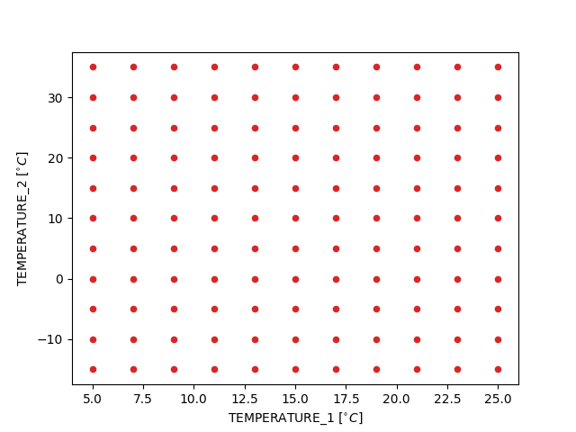
Grid of parameter values ​​resulting from the get_cartesian_product function of the repeat.parametric_study module

The next step is to create a common design_cases table suitable for storing all design cases containing temperature boundary conditions and heat flux calculation results.

design_cases = input_data.copy(deep = True)
design_cases["heat_flux_1"] = pd.NA
design_cases["heat_flux_2"] = pd.NA
design_cases.tail()

Next, we need to run a cycle of model calculations on the REPEAT VISION platform. To do this, we create and execute the solve function in the next cell.

def solve(input_data, design_cases):
    for i, variables in input_data.iterrows():
        with model as md:
            md.run(variables)
            design_cases.loc[i, "heat_flux_2"] = md.get_results("heat_flux_2").iloc[-1]

solve(input_data, design_cases)

In the next step, the heat flux heat_flux_1 is calculated in accordance with the requirements for the machine learning model for further integration into the REPEAT VISION platform.

design_cases.loc[:, "heat_flux_1"] = - design_cases.loc[:, "heat_flux_2"]

Next, you need to save a common design_cases table in case you create other ML models using previously obtained modeling results.

design_cases.to_csv("heat_transfer_data.csv")

To display the calculation results on a grid of parameter values, it is necessary to create an auxiliary function for three-dimensional visualization based on the capabilities of the matplotlib package.

def plot_3d_scatter(table):
    fig = plt.figure()
    ax = fig.add_subplot(projection = "3d")
    ax.scatter(
        table["TEMPERATURE_2"], 
        table["TEMPERATURE_1"], 
        table["heat_flux_2"], 
        marker='o',
        c = 'tab:orange'
      )
    ax.set_xlabel("TEMPERATURE_2 $[^{\circ}C]$")
    ax.set_ylabel("TEMPERATURE_1 $[^{\circ}C]$")
    ax.set_zlabel("heat_flux_2 $[W]$")
    plt.show()

plot_3d_scatter(design_cases)

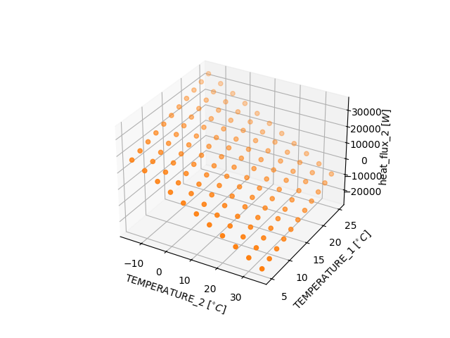
Results of calculating the heat flux heat_flux_2 on the grid of parameter values ​​TEMPERATURE_1 and TEMPERATURE_2

The three-dimensional picture of the distribution of the dependence of heat_flux_2 on TEMPERATURE_1 and TEMPERATURE_2 shows a linear dependence of the heat flux on temperatures, corresponding to the functional dependencies of block №1 Conductive heat transfer, which determines the choice of the architecture of the machine learning model that will be created in the next section.

4.  Creating a machine learning model for thermal conductivity

To create a machine learning model, it is necessary to pre-process the data, dividing it into training data and model testing data.

In the next cell, the results of the heat flux calculation are allocated in a separate variable name heat_flux.

heat_flux = design_cases[["heat_flux_1", "heat_flux_2"]]

Next, we need to create a helper function, get_torch_tensors, to prepare the torch.tensor data structures, since the machine learning model will be created using the PyTorch framework. It is important to note that, in accordance with the requirements for the ML model, the torch.double data type is used when creating the torch.tensor.

def get_torch_tensors(tables : pd.DataFrame):
    total = []
    for table in tables:
        tensors = {}
        for key, values in table.items():
            tensors[key] = torch.tensor(values.to_numpy(), dtype = torch.double).reshape(-1, 1)
        
        total.append(tensors)    
        
    return total

In the next cell, using the train_test_split function of the scikit-learn library, the previously prepared data is split into a training set and a testing set.

input_data_train, input_data_test, heat_flux_train, heat_flux_test = train_test_split(
    input_data, heat_flux, test_size = 0.33, random_state = 42
    )

The next step is to create a machine learning model using the PyTorch framework.

Description of the linear regression model

class LinearModel(nn.Module):
    def __init__(self, temperature_mean, temperature_std):
        super().__init__()
        self.linear = nn.Linear(
            in_features = 2, 
            out_features = 1 
        )
        self.temperature_mean = temperature_mean
        self.temperature_std = temperature_std
        
    def forward(self, TEMPERATURE_1, TEMPERATURE_2):
        x = torch.cat([TEMPERATURE_1, TEMPERATURE_2], dim = 1)
        x = (x - self.temperature_mean) / self.temperature_std
        heat_flux_2 = self.linear(x)
        heat_flux_1 = - heat_flux_2
        return heat_flux_1, heat_flux_2

• Lines 4-7. In the LinearModel model, a layer is created that accepts 2 parameters (temperature boundary conditions) and calculates the result for 1 parameter.

• Lines 8-9. The linear regression model uses additional statistical parameters of temperatures: the mean value temperature_mean and the standard deviation temperature_std.

• Line 11. The forward method takes two arguments as model input parameters corresponding to the temperature boundary conditions: TEMPERATURE_1 and TEMPERATURE_2.

• Line 12. The initial parameters are prepared. The temperature parameters are combined into a common tensor for transfer to the linear layer of the model. The parameters are combined by columns dim = 1.

• Line 13. Temperature values ​​are normalized to unity to ensure the convergence of the process of determining the unknown coefficients of the linear regression model.

• Line 14. The heat flux heat_flux_2 is calculated in accordance with the problem statement.

• Line 15. The heat flux heat_flux_1 is determined in accordance with the ML model requirements for subsequent integration into the REPEAT VISION platform for data exchange with Heat exchange library blocks.

The next cell prepares the means and standard deviations of the temperature boundary conditions using the describe() method of the Pandas library.

summary = input_data_train.describe()
temperature_mean = torch.tensor(summary.loc["mean"].to_numpy(), dtype = torch.double)
temperature_std = torch.tensor(summary.loc["std"].to_numpy(), dtype = torch.double)

The next step is to convert the pandas.DataFrame data structures into torch.tensor structures so that the data can be used later to train the ML model.

input_data_train, input_data_test, heat_flux_train, heat_flux_test = get_torch_tensors((
    input_data_train, input_data_test, heat_flux_train, heat_flux_test
))

Next, the process of training the ML model is carried out.

Description of the model training cycle

torch.manual_seed(42)
model = LinearModel(temperature_mean, temperature_std).double()
criterion = nn.MSELoss()
optimizer = optim.SGD(model.parameters(), lr = 0.1)
num_epochs = 100
model.train()
for epoch in tqdm(range(num_epochs)):
    optimizer.zero_grad()
    outputs = model(**input_data_train)
    loss = criterion(outputs[1], heat_flux_train["heat_flux_2"])
    loss.backward()
    optimizer.step()

• Line 2. Initialization of an instance of the LinearModel model class, switching the model to double-precision mode using the .double() method in accordance with the requirements of the REPEAT VISION platform for ML models.

• Line 3. Initialization of the criterion loss function using the mean squared error.

• Line 4. Initialization of the SGD optimizer to update the model parameters. The learning rate (lr = 0.1) is determined empirically.

• Line 10. During the training process, the loss function calculates the residual for the estimated heat flux value heat_flux_2.

In the next cell, the quality of the created model is assessed using the mean squared error on the test portion of the input_data_test and heat_flux_test data.

model.eval()
with torch.no_grad():
    predictions = model(**input_data_test)
    mse = criterion(predictions[1], heat_flux_test["heat_flux_2"])
    print(f"Mean Squared Error (MSE): {mse.item():.4f}")

At the end of the ML model creation process, the machine learning model is saved in the neutral ONNX format used by the REPEAT VISION platform for integration of approximation models for use in structural modeling.

Description of the settings for saving a model to ONNX format

torch.onnx.export(
    model,
    args = (
        torch.tensor([[5]], dtype = torch.double), 
        torch.tensor([[-15]], dtype = torch.double)
    ),
    f = "ml_heat_transfer.onnx",
    input_names = ["TEMPERATURE_1", "TEMPERATURE_2"],
    output_names = ["heat_flux_1", "heat_flux_2"],    
    )

• Line 2. The first argument passed to the torch.onnx.export() function is the previously trained model model.

• Lines 3-6. The named argument args is passed the default temperature boundary conditions. The data structure used is a 1x1 torch.tensor of type torch.double, in accordance with the requirements of the REPEAT VISION platform for the ML model.

• Lines 7. The named argument f is assigned the name of the saved ONNX format file for subsequent use on the REPEAT VISION platform.

• Lines 8. The named argument input_names is assigned a list of names of temperature boundary conditions for convenient display on the block’s input ports on the REPEAT VISION platform.

• Lines 9. The named argument output_names is assigned a list of names of heat flux calculation results for their convenient display on the block’s output ports on the REPEAT VISION platform.

5.  Integrating a Machine Learning Model into the REPEAT VISION Platform

Finally, you need to upload the ML file of the ml_heat_transfer.onnx model to the REPEAT VISION platform using the Approximation model (Heat exchange) block and transform the original project to the form presented below.

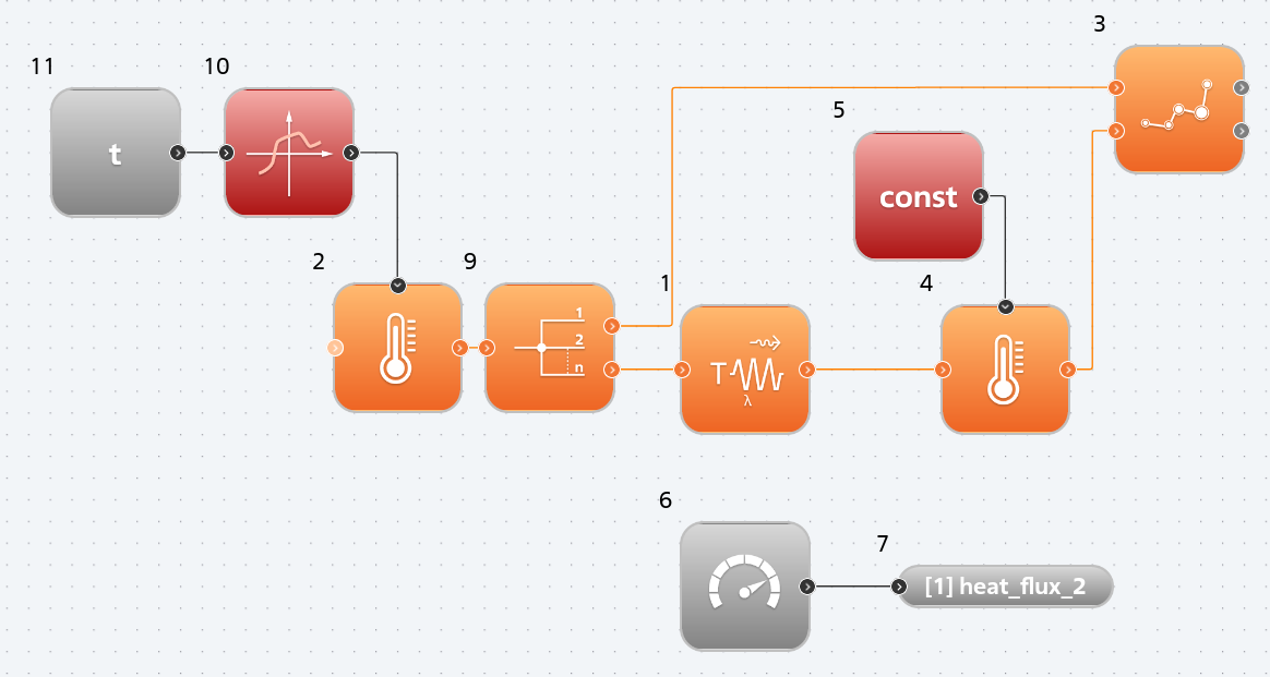
Machine learning model validation scheme for calculating heat flow in the wall of a product part.

The project pictured above allows you to test the machine learning model contained in block №8 Approximation model (Heat exchange).

Hint

Testing of an ML model is performed to independently assess its quality in accordance with the selected model quality criteria.

The project must use the following settings:

Simulation time \([s]\)	Integration step \([ms]\)	Sampling step \([ms]\)
0.5	20	20

Block №10 Single parameter nonlinear function is intended for preparing new data on temperature TEMPERATURE_1, not included in the training set:

Simulation time \([s]\)	Temperature \([^{\circ}C]\)
0.1	2
0.2	10
0.3	35
0.4	27
0.5	1

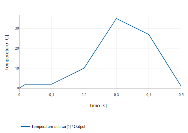
Changing the boundary conditions for temperature using the Nonlinear function of one parameter block.

To test the ML heat conductivity model, the reference heat flow calculation data is generated by block №1 Conductive heat transfer.

At the next step, the dependences of heat flows on time are formed for a comparative analysis of the calculation results of the ML model and block №1 Conductive heat transfer.

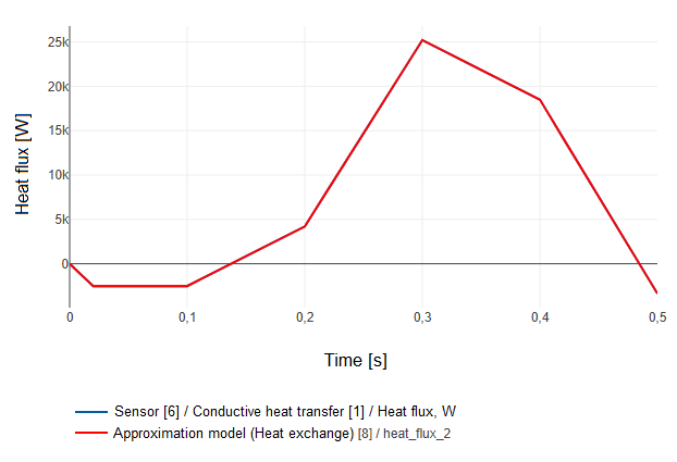
Dependences of heat flows on time for the approximation model and the Thermal conductivity block.

The graphs shown above show that the heat flux values ​​calculated by the ML model match the reference values ​​calculated by block №1 Conductive heat transfer.

6.  Conclusions

As a result of completing this practical guide:

1. You have become familiar with the process of preparing a machine learning model for approximating the stationary process of heat transfer by thermal conductivity in the wall of a part using the REPEAT VISION platform and PyTorch;

2. You have learned how to integrate a model into the REPEAT VISION ML platform using the Approximation model (Heat exchange) block to solve heat exchange and heat transfer problems;

3. You have become familiar with testing a machine learning model both during its creation and during its operation on the REPEAT VISION platform.