Machine learning model of maximum stresses in a gas pipeline branch arising from erosive wear

The how-to guide provides a detailed description of the creation of a machine learning model for approximating the maximum stresses acting in a bend and arising from erosive wear of the inner surface of the bend during the operation of a gas pipeline.

As you read this guide, you will learn:

1. Where and why is a gas pipeline loop needed?

2. The purpose and objectives of modeling the process of operating gas pipelines;

3. Basic steps to create a machine learning model (ML model) using Python to evaluate the erosion process;

4. How to use the ML model with a gas-dynamic model of a gas pipeline on the REPEAT VISION platform.

1.  General information about gas pipelines

Gas pipelines (see figure below) are used at gas fields and are designed to transport gas from wells to an integrated gas treatment unit (IGTU). After undergoing the necessary preparation for transport to the IGTU, the gas enters the main gas pipeline.

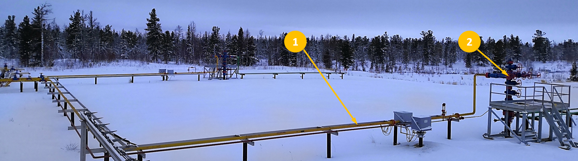
A gas pipeline loop on a cluster of two gas wells.

The gas pipeline (№1 in the figure above) is subject to the following influences during operation:

1. The inner surface of the gas pipeline is loaded with gas pressure and temperature;

2. The outer surface of the gas pipeline is subject to variable temperatures of the external environment.

1.1.  The problem of erosive wear of the gas pipeline

The process of operating a gas well (№2 in the figure above) may be accompanied by the removal of water containing mechanical impurities, which causes erosive wear of the inner surface of the gas pipeline.

The removal of water containing a small amount of mechanical impurities can occur continuously, which makes it possible to create simple semi-empirical analytical methods for predicting erosive wear.

Erosive wear can also be cyclical in nature with periodic removal of water and mechanical impurities.

There are also very dangerous sudden releases of mechanical impurities with large quantities of water, which can lead to unexpected and significant wear of gas pipeline components.

The most vulnerable element of a gas pipeline is the first branch, if you count from the wellhead of the gas well (№2 in the figure above).

1.2.  Ways to reduce risk

To reduce the risk of incidents and accidents due to erosive wear of the gas pipeline, a comprehensive solution is required, including:

1. Application of physical and mathematical modeling of the process of operation of a pipeline system and its control system;

2. Application of automated diagnostic tools for the technical condition of gas pipeline elements;

3. Implementation of automated control systems for gas well operation processes using the results of mathematical modeling of the current technical condition of the gas pipeline.

2.  Diagnostic tools for the technical condition of gas pipelines

Automated diagnostic tools for the technical condition of gas pipeline components required to monitor the erosion process include the following systems:

1. Flow control systems;

2. External temperature sensors and gas pressure and temperature control systems;

3. Intrusive erosion measurement sensors and acoustic sand monitoring systems;

4. Point and distributed thickness measurement systems.

3.  The purpose and objectives of modeling the operation process of gas pipelines

Objective: To improve the company’s production efficiency and prevent accidents at industrial facilities.

Modeling tasks:

1. Calculation of strength parameters based on current data on the technical condition of gas pipelines;

2. Calculation of the parameters of the collection system for compliance with the technical project for field development;

3. Ensuring maximum gas production during peak seasonal periods (winter, demand) and minimum production (summer);

4. Ensuring optimal operating parameters of the collection system during unplanned shutdown of wells or when well operating modes do not correspond to the design ones;

5. Determination of parameters of the collection system when changing the input parameters of the gas and condensate treatment system.

The solution to problem #1 is presented in the next section. The remaining problems are solved by modeling pipeline systems using REPEAT VISION and solving global and local optimization problems.

4.  Description of the task

Perform an assessment of the stress-strain state (SSS) of the branch based on the initial data and boundary conditions.

The machine learning model is created based on a data table of the static strength calculation results for the branch model. Each row in the data table represents a separate design case. Each design case includes:

1. Initial data and boundary conditions:

   1. Minimum wall thickness,

   2. Gas pressure

   3. Gas temperature,

   4. Ambient temperature,

2. Calculation result SSS: Maximum stresses according to von Mises.

The calculation cases are based on the technological regulations of a specific field:

1. Gas pressure varies in the range: from 8.5 to 6.0 \([MPa]\),

2. The gas temperature varies in the range: from 7 to 20 \([^{\circ}C]\),

3. The ambient temperature varies in the range: from -55 to 40 \([^{\circ}C]\),

4. The design cases include minimum branch wall thicknesses from 6.45 to 4.9 \([mm]\).

The result of the calculation of the static strength of one of the design cases is the von Mises stress distribution shown in the figure below.

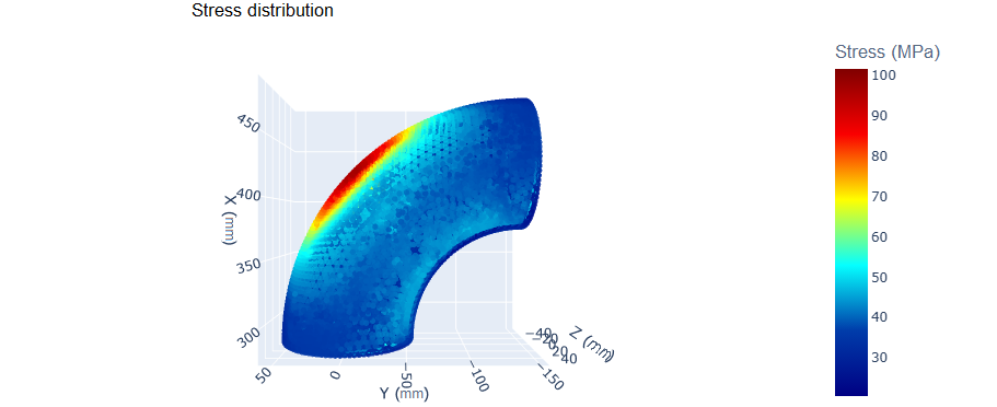
An example of von Mises stress distribution in a bend.

For each result of the calculation of stresses acting in the branch, shown in the figure above, the maximum value is selected and entered into the table of calculation results.

5.  Preparing a table of calculation cases

The calculation of the static strength of the bend is performed in a software package that implements the finite element method (FEM).

5.1.  Static strength model

To determine the SSS of the branch, the influence of the entire gas pipeline-loop and the associated support structures a cluster of two gas wells was taken into account.

Linear sections of the gas pipeline loop and supporting structures were modeled in the beam approximation.

The bends and tees were modeled using volumetric FE.

5.2.  The main stages of data preparation

The preparation of the table of design cases is reduced to an automated process of parametric studies of the static strength of the bend, which in itself is a separate engineering task.

Hint

If you need more information and skills in performing parametric studies, please check out our how-to guide on this topic.

The main stages of the parametric study process are shown in the figure below.

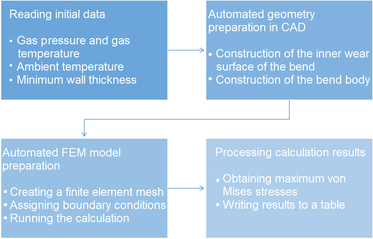
The process of data preparation based on the modeling of the static strength of the bend.

This process was repeated approximately 6000 times in the parametric study workflow to obtain the required table of design cases for subsequent creation of the machine learning model.

6.  Building a neural network model

Note

You can download the Jupyter notebook file and the requirements.txt file to create the necessary virtual environment if you want to quickly run the code in this tutorial on your personal computer.

Additionally, you will need data for training the model and (optionally) data for visualization of one calculation result.

You can also download the model file and immediately use it in a project on the REPEAT VISION platform using the Approximation model block.

The model will be written using the Python language and the PyTorch framework, so basic knowledge of this language and skills in working with PyTorch are required.

Important

Please note that to install a GPU-enabled version of PyTorch that is compatible with your CUDA version, you need to visit the official website.

In addition, to solve the problem, many libraries that are generally accepted for the corresponding subtasks are used:

• NumPy and Pandas — working with arrays, linear algebra, and processing tabular data, respectively.

• Matplotlib, Seaborn — visualization of static graphs to monitor the quality of model performance.

• Plotly - interactive graphs for visual representation of the object of study.

• scikit-learn — metrics calculation and data partitioning.

Перед началом подготовки ML модели необходимо установить Python, а также требуется установить пакеты для работы с данными и создания ML модели. Для этого необходимо выполнить в командной строке вашего компьютера следующие команды и продолжить работу в Jupyter ноутбуке.

Bash

mkdir ml_branch_stress
cd ml_branch_stress
python -m venv repeat_ml.
source repeat_ml/bin/activate
python -m pip install numpy pandas scikit-learn onnx onnxscript 
python -m pip install seaborn matplotlib plotly 
python -m pip install jupyterlab tqdm ipywidgets netron
python -m pip install torch --index-url https://download.pytorch.org/whl/cpu

jupyter lab

PowerShell

mkdir ml_branch_stress
cd ml_branch_stress
python -m venv repeat_ml.
repeat_ml\Scripts\Activate.ps1
python -m pip install numpy pandas scikit-learn onnx onnxscript 
python -m pip install seaborn matplotlib plotly 
python -m pip install jupyterlab tqdm ipywidgets netron
python -m pip install torch --index-url https://download.pytorch.org/whl/cpu

jupyter lab

First of all, we import the necessary libraries for creating neural networks, building visualizations, and subsequent import into the ONNX format.

Importing libraries

import numpy as np
import pandas as pd

import seaborn as sns
import matplotlib.pyplot as plt
import plotly.graph_objects as go

import torch
import torch.nn as nn
import torch.optim as optim
from torch.utils.data import Dataset, DataLoader

from sklearn.model_selection import train_test_split
from sklearn.metrics import (mean_squared_error, 
                             mean_absolute_error,
                             mean_absolute_percentage_error,
                             r2_score)

from tqdm.notebook import tqdm
from typing import Tuple, List, Dict, Union

To improve reproducibility and utilization of the available device, it is necessary to fix random number generation and graphics accelerator availability.

Reproducibility and design

SEED = 42
torch.manual_seed(SEED)
np.random.seed(SEED)

device = torch.device('cuda' if torch.cuda.is_available() else 'cpu')
print(device)

6.1.  Data exploration

To visualize the stress distribution in the branch, we visualize the three-dimensional distribution of points using interactive 3D visualization with Plotly.

Stress visualization

def branch_plot(df: pd.DataFrame) -> go.Figure:
    """
    Создает 3D визуализацию распределения напряжений.
    
    Параметры:
        df: pd.DataFrame
            DataFrame с данными о координатах и напряжениях
    Возвращает:
        go.Figure: Объект графика Plotly
    """
    marker_config = dict(
        size=3,
        color=df['Stress'],
        colorscale='Jet',
        opacity=0.8,
        colorbar=dict(title="Напряжение (МПа)")
    )
    hover_template = (
        '<b>Узел</b>: %{customdata}<br>'
        '<b>X</b>: %{x:.2f} мм<br>'
        '<b>Y</b>: %{y:.2f} мм<br>'
        '<b>Z</b>: %{z:.2f} мм<br>'
        '<b>Напряжение</b>: %{marker.color:.2f} МПа'
    )
    fig = go.Figure(
        data=[
            go.Scatter3d(
                x=df['X'],
                y=df['Y'],
                z=df['Z'],
                mode='markers',
                marker=marker_config,
                hovertemplate=hover_template,
                customdata=df['Node']
            )
        ]
    )
    scene_config = dict(
        xaxis_title='X (мм)',
        yaxis_title='Y (мм)',
        zaxis_title='Z (мм)',
        aspectmode='data',
        camera=dict(
            eye=dict(x=0, y=0, z=2.5),
            center=dict(x=0, y=0, z=0),
            up=dict(x=0, y=1, z=0)
        )
    )
    margin_config = dict(l=0, r=0, b=0, t=30)
    fig.update_layout(
        title='Распределение напряжений',
        scene=scene_config,
        margin=margin_config
    )

    return fig

As a result, for a randomly selected file containing the results of a numerical experiment, a set of points will be plotted. The color of the points will represent the voltage magnitude, and the familiar \(X, Y, Z\) axes will be used. We’ll create the visualization by executing the following code:

Building stress visualization

df = pd.read_csv('stress_branch.csv')
fig = branch_plot(df)
fig.show()

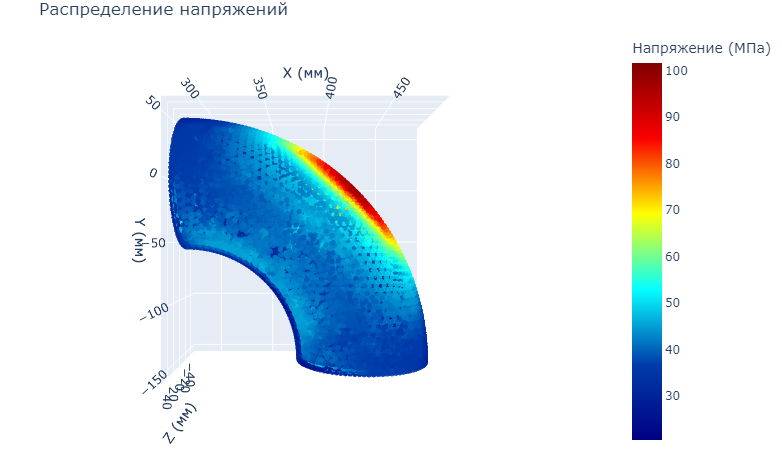
Stress distribution in the branch.

After processing these types of files, the data needed for training was aggregated into a table. Of all the von Mises stress values ​​calculated in the bend, the maximum value was recorded in the table.

The final table for setting the regression problem has the following parameters:

• Input parameters (features):

  • Pressure varies in the range: 6.0 - 8.5 \([MPa]\).

  • Gas temperature (gas_temperature) varies in the range: 7.0 - 20.0 \([^{\circ}C]\).

  • Ambient temperature (ambient_temperature) varies in the range: -55.0 - 40.0 \([^{\circ}C]\).

  • Minimum wall thickness (wall_thickness_min), varies in the range: 4.90 - 6.45 \([mm]\).

• Target variable:

  • The maximum von Mises stress in the structure (stress_max) varies in the range: 45.31 - 140.40 \([MPa]\).

Distribution of training data

df = pd.read_csv('branch_data.csv')
df.describe()

To display data directly in the form of a table, with columns divided into features and a target variable, you can use the following code:

Displaying training data

features = ['pressure', 'gas_temp', 'ambient_temp', 'wall_thickness']
target = 'stress_max'

df[features + [target]].head()

6.2.  Data preparation

To efficiently work with data, PyTorch uses a special class, StressDataset, which inherits from torch.utils.data.Dataset. The parent class is abstract and requires the implementation of two main methods: __len__() and __getitem__(). Ultimately, this class performs several important functions:

1. Encapsulates data loading and preprocessing logic. In this case, it converts data to a torch.Tensor and transfers it to the required device.

2. Provides a consistent data access interface that simplifies working with a model that meets the requirements for integration into REPEAT VISION.

3. Allows you to work efficiently with large data sets by loading them in portions, which is implemented in this case using features as an example.

4. Simplifies integration with DataLoader for batching and shuffling data.

Definition of the StressDataset class

class StressDataset(Dataset):
    """
    Класс датасета для обучения модели.
    """
    def __init__(
        self,
        X: np.ndarray,
        y: np.ndarray,
        device: torch.device = torch.device('cpu')
    ) -> None:
        """
        Инициализация набора данных.

        Параметры:
            X: np.ndarray
                Массив входных признаков
            y: np.ndarray
                Массив целевых значений
            device: torch.device
                Устройство для вычислений
        """
        super().__init__()
        self.device = device
        self.X = X
        self.y = torch.FloatTensor(y, device=self.device).reshape(-1, 1)
    
    def __len__(self) -> int:
        """
        Методы получения количества элементов.
        
        Возвращает:
            int: Количество элементов
        """
        return len(self.X)
    
    def __getitem__(self, idx: int) -> Tuple[Tuple[torch.Tensor, ...], torch.Tensor]:
        """
        Возвращает пару (признаки, целевое значение) для заданного индекса.
        
        Параметры:
            idx: int
                Индекс образца
            
        Возвращает:
            Tuple[Tuple[torch.Tensor, ...], torch.Tensor]: 
                Кортеж из кортежа признаков и целевого значения
        """
        return (
            tuple(torch.Tensor([feature], device=self.device) 
                  for feature in self.X[idx]),
            self.y[idx]
        )

Important

It is important to note that each feature is returned as a separate tensor, which is important for export to ONNX and integration with REPEAT VISION.

Let’s use the created class to prepare data for training.

Preparing data for training and testing

X = df[features].values
y = df[target].values

X_train, X_test, y_train, y_test = train_test_split(
    X, y,
    test_size=0.2,
    random_state=42
)

train_dataset = StressDataset(X_train, y_train, device)
test_dataset = StressDataset(X_test, y_test, device)

batch_size = 64
train_loader = DataLoader(
    train_dataset, 
    batch_size=batch_size, 
    shuffle=True
)
test_loader = DataLoader(
    test_dataset, 
    batch_size=batch_size, 
    shuffle=False
)

The result of executing this code is:

• Lines 1-2. Separation of numerical values ​​of features and the target variable.

• Lines 4-8. Splitting into training and test samples.

• Line 10-11. Creating instances of the StressDataset class for training and testing

• Line 13-23. Creating instances of the DataLoader class to efficiently load data in batches.

6.3.  Neural network architecture

The problem contains four input features: pressure (pressure), gas temperature (gas_temp), ambient temperature (ambient_temp), and wall thickness (wall_thickness). These are all combined into a single vector of size 4. The output is a single numerical value (the predicted maximum stress), making the problem an example of a regression problem:

\[ f: \mathbb{R}^4 \rightarrow \mathbb{R} \]

where:

\[ f(p, t_g, t_a, w) = \sigma_{max} \]

where:

\(p\) - давление;

\(t_g\) - gas temperature;

\(t_a\) - ambient temperature;

\(w\) - wall thickness;

\(\sigma_{max}\) - maximum voltage.

Various models can be applied to tabular data, from classical machine learning to deep neural networks. In this case, the MLP (Multi Layer Perceptron) model is used.

• The model’s architecture is a three-layer fixed-depth MLP, where the size of the hidden layers is configured during initialization. This structure provides sufficient capacity to approximate nonlinear relationships in the data.

Matrix representation of a three-layer MLP model with 4 input channels, 1 output channel and a hidden state \( h \):

\[\begin{split} \begin{align*} h_1 &= \text{ReLU}(\text{LayerNorm}(W_1 x + b_1)) \\ h_2 &= \text{ReLU}(\text{LayerNorm}(W_2 h_1 + b_2)) \\ h_3 &= \text{ReLU}(\text{LayerNorm}(W_3 h_2 + b_3)) \\ y &= W_4 h_3 + b_4 \end{align*} \end{split}\]

where:

• \(x \in \mathbb{R}^4\) - input feature vector

• \(W_1 \in \mathbb{R}^{h \times 4}, b_1 \in \mathbb{R}^{h}\) - weights and biases of the first layer

• \(W_2 \in \mathbb{R}^{h \times h}, b_2 \in \mathbb{R}^{h}\) - weights and biases of the second layer

• \(W_3 \in \mathbb{R}^{h \times h}, b_3 \in \mathbb{R}^{h}\) - weights and biases of the third layer

• \(W_4 \in \mathbb{R}^{1 \times h}, b_4 \in \mathbb{R}\) - weights and biases of the output layer

• \(y \in \mathbb{R}\) is the output value (predicted voltage)

The model uses several ideas:

• To stabilize training, the model uses pre-computed statistics (mean and std) from the training dataset. Normalizing the input features in the forward method allows each example to be brought to a single distribution without requiring a separate normalizer, which would complicate import into REPEAT VISION.

• A combination of Dropout, L2 regularization (weight decay) and early stopping (early stopping) is used as regularization. The ReLU activation function was chosen based on data analysis, although smoother variants could be used alternatively. The Kaiming method is used to initialize the weights, which stabilizes the variance of the layer outputs and prevents gradient problems. The biases are initialized to zeros since they learn themselves quickly.

• Instead of the popular BatchNorm, preference is given to LayerNorm, which ensures more stable training on consistent data with significant statistical differences between batches.

All the described ideas are implemented in the StressNet class. This architecture provides a good balance between model capacity and regularization, which is especially important when working with small datasets, as in this problem.

Definition of the StressNet class

class StressNet(nn.Module):
    """
    Нейронная сеть.
    """
    def __init__(
        self,
        input_size: int = 4,
        hidden_size: int = 32,
        mean: torch.Tensor = torch.zeros(4),
        std: torch.Tensor = torch.ones(4),
        dropout_rate: float = 0.2
    ) -> None:
        """
        Инициализация модели.
        
        Параметры:
            input_size: int
                Размер входного слоя
            hidden_size: int
                Размер скрытых слоев
            mean: torch.Tensor
                Средние значения для нормализации
            std: torch.Tensor
                Стандартные отклонения для нормализации
            dropout_rate: float
                Вероятность отключения нейронов
        """
        super().__init__()
        
        self.fc1 = nn.Linear(input_size, hidden_size)
        self.norm1 = nn.LayerNorm(hidden_size)
        self.fc2 = nn.Linear(hidden_size, hidden_size)
        self.norm2 = nn.LayerNorm(hidden_size)
        self.fc3 = nn.Linear(hidden_size, hidden_size)
        self.norm3 = nn.LayerNorm(hidden_size)
        self.out = nn.Linear(hidden_size, 1)

        self.act = nn.ReLU()
        self.dropout = nn.Dropout(dropout_rate)

        self.mean = mean
        self.std = std

        self.apply(self._init_weights)

    def _init_weights(self, module: nn.Module) -> None:
        """
        Инициализация весов слоев.
        
        Параметры:
            module: nn.Module
                Модуль для инициализации весов
        """
        if isinstance(module, nn.Linear):
            nn.init.kaiming_uniform_(
                module.weight,
                nonlinearity='relu'
            )
            nn.init.zeros_(module.bias)

    def forward(
        self,
        pressure: torch.Tensor,
        gas_temp: torch.Tensor,
        ambient_temp: torch.Tensor,
        wall_thickness: torch.Tensor
    ) -> torch.Tensor:
        """
        Прямой проход через сеть.
        
        Параметры:
            pressure: torch.Tensor
                Давление
            gas_temp: torch.Tensor
                Температура газа
            ambient_temp: torch.Tensor
                Температура окружения
            wall_thickness: torch.Tensor
                Толщина стенки
            
        Возвращает:
            torch.Tensor: Предсказанное значение максимального напряжения
        """
        batch_size = pressure.shape[0]
        
        x = torch.cat([
            pressure.view(batch_size, -1),
            gas_temp.view(batch_size, -1),
            ambient_temp.view(batch_size, -1),
            wall_thickness.view(batch_size, -1)
        ], dim=1)

        x = (x - self.mean) / self.std

        x = self.fc1(x)
        x = self.norm1(x)
        x = self.act(x)
        x = self.dropout(x)

        x = self.fc2(x)
        x = self.norm2(x)
        x = self.act(x)
        x = self.dropout(x)

        x = self.fc3(x)
        x = self.norm3(x)
        x = self.act(x)
        x = self.dropout(x)

        return self.out(x)

• Lines 30-39. Declaring three layers with LayerNorm and Dropout for regularization.

• Lines 41-42 Since the input data is normalized within the model, mean and std are passed to the constructor.

• Lines 44. The initialization of the weights is applied (lines 46-59).

• Lines 61-110 The main method, forward, takes the required input parameters, combines them into a single tensor, and then passes it through all the layers in the required order.

After defining the model architecture, it is necessary to initialize the model itself and configure the optimizer and criterion (loss function).

In this case, the following configuration is used:

• The hidden layer size (hidden_size) is set to 512 neurons.

• The dropout rate is 0.2

• Statistics from the training set are used to normalize the input data

• The mean square error (MSE) is chosen as the loss function.

• AdamW optimizer with learning rate 5e-4 and L2 regularization 1e-4

Announcement of the task and general statement of the task

hidden_size = 512
dropout_rate = 0.2

stats = pd.DataFrame(df[features])
mean = torch.tensor(stats.mean().values, dtype=torch.float32)
std = torch.tensor(stats.std().values,  dtype=torch.float32)

model = StressNet(
    input_size=len(features),
    mean=mean,
    std=std,
    hidden_size=hidden_size,
    dropout_rate=dropout_rate 
)

criterion = nn.MSELoss()
optimizer = optim.AdamW(model.parameters(), lr=5e-4, weight_decay=1e-4)

6.4.  Model training

The train_model function is designed to train a neural network using the gradient descent method. Here are the main components and steps of the function:

• Preparation:

  • Transfer the model to the specified device.

  • Initializing lists for tracking losses.

  • Setting up early stopping.

• Learning cycle:

  • Learning from training data.

  • Validation on test data.

  • Tracking the best model.

  • Checking early stopping conditions.

• Monitoring:

  • Tracking the value of the loss function.

  • Saving the best model.

  • Conclusion of learning progress.

This implementation provides stable model training with early stopping capability to prevent overfitting.

Definition of the train_model function

def train_model(
    model: nn.Module,
    train_loader: DataLoader,
    val_loader: DataLoader,
    criterion: nn.Module,
    optimizer: optim.Optimizer,
    epochs: int,
    device: torch.device = torch.device('cpu'),
    patience: int = 20
) -> Tuple[nn.Module, List[float], List[float]]:
    """
    Обучает модель нейронной сети.
    
    Параметры:
        model: nn.Module
            Модель нейронной сети для обучения
        train_loader: DataLoader
            Загрузчик данных для обучающей выборки
        val_loader: DataLoader
            Загрузчик данных для валидационной выборки
        criterion: nn.Module
            Функция потерь
        optimizer: optim.Optimizer
            Оптимизатор для обновления весов
        epochs: int
            Количество эпох обучения
        device: torch.device
            Устройство для вычислений (CPU/GPU)
        patience: int
            Количество проведенных эпох без улучшения, достаточное для ранней остановки обучения
        
    Возвращает:
        Tuple[nn.Module, List[float], List[float]]: Обученная модель, 
            список потерь на обучающей выборке, список потерь на валидационной выборке
    """
    model.to(device)
    
    train_losses = []
    val_losses = []
    
    best_val_loss = float('inf')
    no_improvement = 0
    best_model_state = None
    
    for epoch in tqdm(range(epochs), desc='Training'):
        model.train()
        train_loss = 0.0
        
        for inputs, targets in train_loader:
            optimizer.zero_grad()
            
            outputs = model(*inputs)
            loss = criterion(outputs, targets)
            
            loss.backward()
            optimizer.step()
            
            train_loss += loss.item() * targets.size(0)
            
        train_loss = train_loss / len(train_loader.dataset)
        train_losses.append(train_loss)
        
        model.eval()
        val_loss = 0.0
        
        with torch.no_grad():
            for inputs, targets in val_loader:
                outputs = model(*inputs)
                loss = criterion(outputs, targets)
                
                val_loss += loss.item() * targets.size(0)
                
        val_loss = val_loss / len(val_loader.dataset)
        val_losses.append(val_loss)
        
        if epoch % 10 == 0:
            print(
                f'Epoch {epoch+1}/{epochs}, '
                f'Train Loss: {train_loss:.6f}, '
                f'Val Loss: {val_loss:.6f}'
            )
        
        if val_loss < best_val_loss:
            best_val_loss = val_loss
            no_improvement = 0
            best_model_state = model.state_dict().copy()
        else:
            no_improvement += 1
            if no_improvement >= patience:
                print(f'Early stopping at epoch {epoch+1}')
                model.load_state_dict(best_model_state)
                break
    
    return model, train_losses, val_losses

• Lines 49-58. The main training loop with loss calculation on the training dataset.

• Lines 66-71. Model validation and loss calculation on the validation set.

• Lines 83-92. Early stopping and best model retention logic.

To train the model, you need to call the train_model function, passing it the previously created parameters and entities correctly.

Calling the train_model function

model, train_losses, val_losses = train_model(
    model=model,
    train_loader=train_loader,
    val_loader=test_loader,
    criterion=criterion,
    optimizer=optimizer,
    epochs=500,
    device=device,
    patience=10
)

6.5.  Model evaluation

The ‘evaluate_model’ function is used to evaluate the performance of a trained neural network on a test dataset. It performs the following steps:

1. Preparing the model:

   • Puts the model into evaluation mode (model.eval()).

   • Disables gradient calculation to optimize memory.

2. Data processing:

   • Iterates through all batches in DataLoader.

   • Gets the model’s predictions.

   • Collects real values ​​and predictions into lists.

3. Metrics calculation:

   • MSE (Mean Squared Error) - root mean square error.

   • RMSE (Root Mean Squared Error) is the root of the root mean square error.

   • MAPE (Mean Absolute Percentage Error) - mean absolute percentage error.

   • MAE (Mean Absolute Error) - mean absolute error.

   • R² (R-squared) - coefficient of determination.

Defining the evaluate_model function

def evaluate_model(
    model: nn.Module,
    data_loader: DataLoader,
    criterion: nn.Module,
    device: torch.device = torch.device('cpu')
) -> Dict[str, Union[float, np.ndarray]]:
    """
    Оценивает производительность модели на заданном наборе данных.
    
    Параметры:
        model: nn.Module
            Модель PyTorch для оценки
        data_loader: DataLoader
            DataLoader с данными для оценки
        criterion: nn.Module
            Функция потерь
        device: torch.device
            Устройство для вычислений
        
    Возвращает:
        Dict[str, Union[float, np.ndarray]]: Словарь с метриками оценки
        и результатами предсказаний
    """
    model.to(device)
    model.eval()
    
    all_targets = []
    all_predictions = []
    total_loss = 0.0
    
    with torch.no_grad():
        for inputs, targets in data_loader:
            outputs = model(*inputs)
            loss = criterion(outputs, targets)
            total_loss += loss.item() * targets.size(0)
            
            all_targets.extend(targets.cpu().numpy())
            all_predictions.extend(outputs.cpu().numpy())
    
    all_targets = np.array(all_targets).flatten()
    all_predictions = np.array(all_predictions).flatten()
    
    mse = mean_squared_error(all_targets, all_predictions)
    rmse = np.sqrt(mse)
    mape = mean_absolute_percentage_error(all_targets, all_predictions)
    mae = mean_absolute_error(all_targets, all_predictions)
    r2 = r2_score(all_targets, all_predictions)
    
    avg_loss = total_loss / len(data_loader.dataset)
    
    return {
        'loss': avg_loss,
        'mse': mse,
        'rmse': rmse,
        'mape': mape,
        'mae': mae,
        'r2': r2,
        'targets': all_targets,
        'predictions': all_predictions
    }

In this implementation, many different metrics of the regression problem are considered in order to obtain the most complete understanding of the quality and accuracy of the problem solution.

To get all the metrics, simply run the following code:

Calling the evaluate_model function

test_results = evaluate_model(model, test_loader, criterion, device)

print("Test metrics:")
print(f"MSE: {test_results['loss']:.3f}")
print(f"RMSE: {test_results['rmse']:.3f}")
print(f"MAPE: {test_results['mape']*100:.3f}%")
print(f"MAE: {test_results['mae']:.3f}")
print(f"R^2: {test_results['r2']:.3f}")

This code will output the results of the model testing.

Metrics	Meaning	Interpretation
MSE	5.281	Root mean square error
RMSE	2.298	Root of the mean square error
MAPE	1.066%	Mean absolute percentage error
MAE	0.814	Mean absolute error
R²	0.987	Coefficient of determination

6.6.  Visualization of results

The visualize_results function is designed to visualize the dynamics of the change in the loss function on the training and validation samples and to construct an error histogram.

Defining the visualize_results function

def visualize_results(
    train_losses: List[float],
    val_losses: List[float],
    test_results: Dict[str, np.ndarray]
) -> None:
    """
    Визуализирует результаты обучения модели.
    
    Параметры:
        train_losses: List[float]
            Список значений функции потерь на обучающей выборке
        val_losses: List[float]
            Список значений функции потерь на валидационной выборке
        test_results: Dict[str, np.ndarray]
            Словарь с результатами тестирования модели
    """
    _, (ax1, ax2) = plt.subplots(1, 2, figsize=(12, 4))
    
    ax1.plot(train_losses, label='Train Loss')
    ax1.plot(val_losses, label='Val Loss')
    ax1.set_xlabel('Epoch')
    ax1.set_ylabel('Loss')
    ax1.legend()
    ax1.grid(True)
    
    errors: np.ndarray = test_results['predictions'] - test_results['targets']
    sns.histplot(errors, bins=30)
    ax2.set_xlabel('Error')
    ax2.set_ylabel('Frequency')
    ax2.grid(True)
    
    plt.tight_layout()
    plt.show()

Let’s call this function.

Calling the visualize_results function

visualize_results(train_losses, val_losses, test_results)

As a result, we have two graphs:

• The first is the dynamics of the loss function during training and validation.

• The second is a histogram of the distribution of prediction errors.

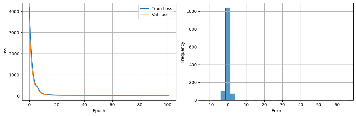
Graphs of changes in the value of the loss function and the distribution of errors.

6.7.  Exporting a model to ONNX

The export_to_onnx function is designed to export a trained PyTorch model to the ONNX format. The function takes into account the need to convert to double mode and takes into account the names of the input and output parameters.

Definition of the export_to_onnx function

def export_to_onnx(
    model: nn.Module,
    features: List[str],
    target: str,
    output_path: str = "stress_model.onnx"
) -> None:
    """
    Экспортирует PyTorch модель в формат ONNX.
    
    Args:
        model: nn.Module
            PyTorch модель для экспорта
        features: List[str]
            Список имен входных признаков
        target: str
            Имя целевой переменной
        output_path: str
            Путь для сохранения ONNX модели
    """
    model.eval()
    model.double()
    
    dummy_inputs: Dict[str, torch.Tensor] = {
        feature: torch.zeros(1, 1, dtype=torch.float64)
        for feature in features
    }
    
    torch.onnx.export(
        model,
        dummy_inputs,
        output_path,
        input_names=features,
        output_names=[target],
        opset_version=12,
        dynamo = False
        )
    
    print(f"Model exported to {output_path}.")

To configure a previously trained model, it is necessary to pass it to the previously declared model and the names of the features and target variable for correct display in REPEAT VISION.

Calling the export_to_onnx function

export_to_onnx(model, features, target)

In the next step, the saved model will be imported into the REPEAT VISION platform in the gas pipeline project to perform interdisciplinary modeling.

7.  The REPEAT VISION platform’s gas pipeline project

The figure below shows a project on the REPEAT VISION platform for modeling a gas pipeline using blocks from the Pneumatics, Automation, and External models libraries. This model of gas pipeline-loop allows:

1. Calculate the parameters of the collection system to ensure compliance with the technical design for the field development;

2. Determine the parameters of the collection system when changing the input parameters of the gas and condensate treatment system.

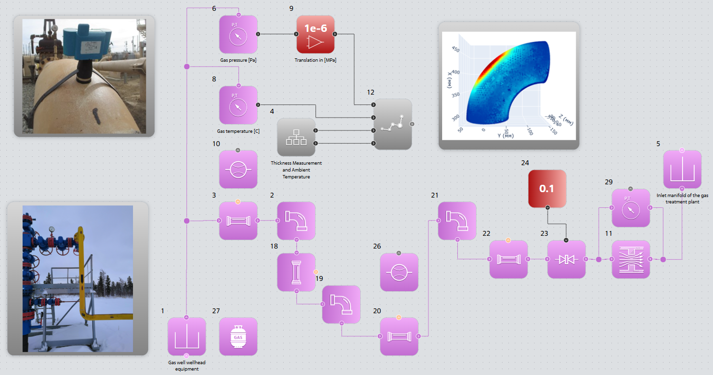
Gas pipeline project on the REPEAT VISION platform.

Within the framework of a single project, based on current data from diagnostics of the technical condition of the gas pipeline-loop, the calculation of von Mises stresses of the branch is also performed using the block №12 Approximation model and the machine learning model imported into this block.

The project shown above allows:

1. Perform computational experiments on machine learning models,

2. In a general interdisciplinary model develop a control system for the technological process of gas production, taking into account the assessment of the maximum von Mises stresses in the branch;

3. Using Modbus blocks, it is possible to create digital twins of gas pipelines for the stage of their operation, connecting thickness measurement systems, pressure, temperature and gas flow measurement systems to the model.

7.1.  Results of computational experiments

The dynamics of the decrease in the wall thickness of the bend is shown in the figure below.

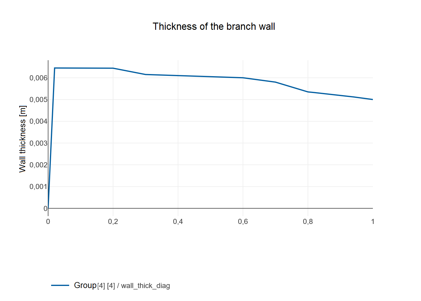
Dynamics of reduction of minimum wall thickness of the bend.

A decrease in the thickness of the branch wall, as well as changes in the ambient temperature while maintaining a constant gas pressure, lead to an increase in stress in the branch, the approximate results of which are shown in the next figure.

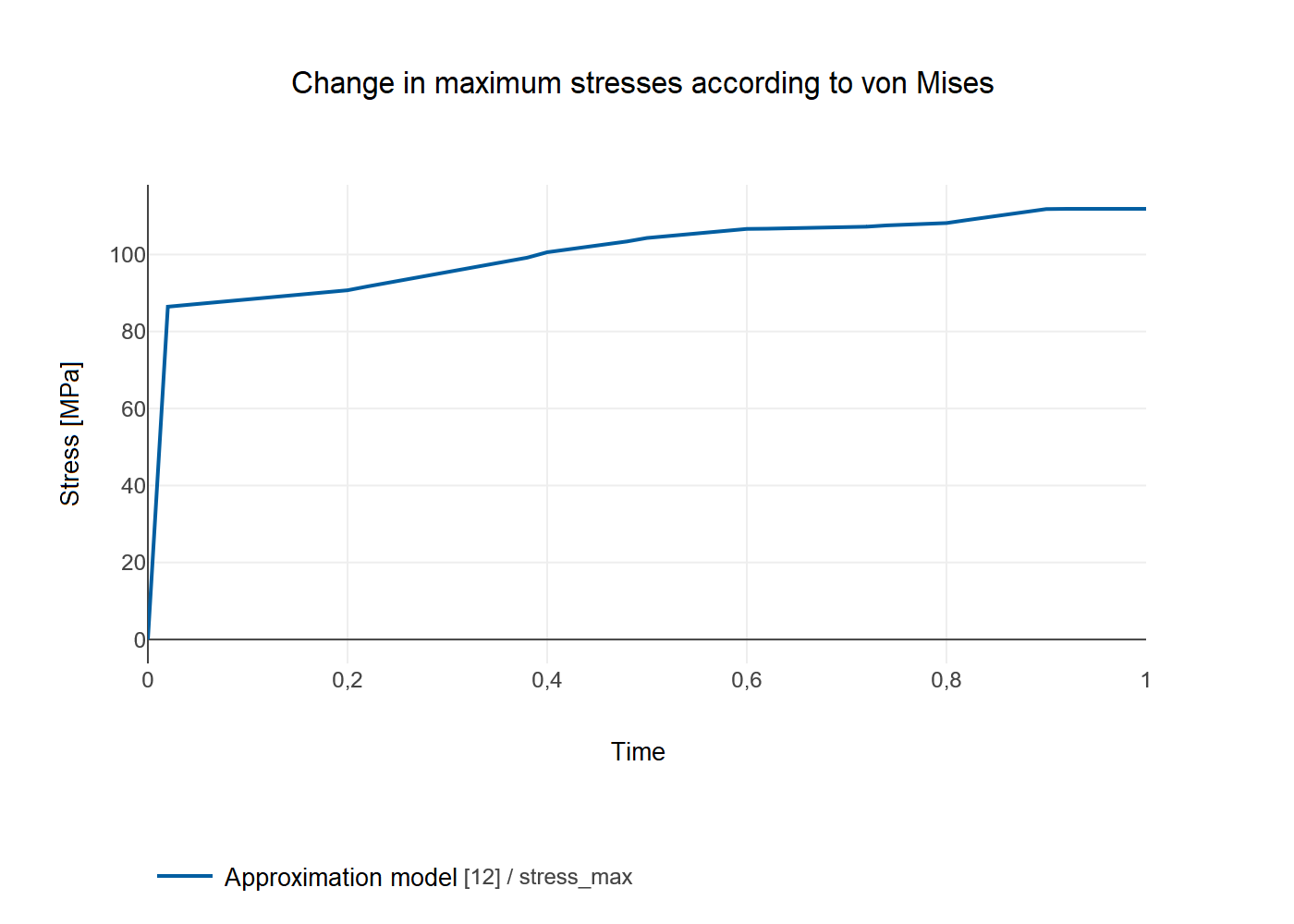
Dynamics of increase of maximum von Mises stresses in a bend.

8.  Conclusions

Integration of machine learning models into the REPEAT VISION platform:

1. Expands the range of tasks to be solved in system modeling and in the creation of digital twins of complex systems;

2. Provides the use of FVM and FEM models of large dimensions, as well as models based on the results of diagnostics of operating systems;

3. Compared to direct integration with external engineering software: eliminates the risk of errors due to problems with the convergence of the FEM (FVM) model calculation, significantly increases the speed of structural design calculation.