Application of Kalman filter for evaluation of measurement results

Measurement data (for example, coordinates of the aircraft, data on weather states of the environment surrounding the product, or parameters of the current technical state of the product) always contain measurement errors. Measurement errors (or data noise) and incomplete data make it difficult to calculate the current technical state of the product.

The Kalman filter allows to solve problems of evaluating measurement results containing noise or errors in order to further use the measurement results in control systems, as well as to calculate the current technical state of products at the stage of their operation.

This practical guide includes:

• Summary of the Kalman filter,

• Description of the basic steps for implementing the Kalman filter on the REPEAT VISION platform using the example of evaluating the pressure sensor measurements.

1.  Kalman filter

The Kalman filteris a mathematical algorithm for modeling linear dynamical systems whose state changes over time.[1] The[1]state of the system refers to the temperature, process pressure, spatial coordinates of the observed object, and other measurable states of the system.

The representation of a linear dynamical system of states in space is expressed by the equation (1).

(1)\[\mathbf x_k = \mathbf{Fx}_{k-1} + \mathbf B_k\mathbf u_k + \mathbf{w_k}\]

In the equation (1) \(\mathbf x_k\) the vector of the current state of the system at the time \(t_k\), \(\mathbf x_{k-1}\) - 1is the vector of the previous state of the system at the time \(t_{k-1}\);

\(\mathbf F\) - is the system state transition matrix. The matrix \(\mathbf F\) - discrete and depicts a system of linear equations that go from state \(\mathbf x_{k-1}\) to state \(\mathbf x_k\) a discrete time step \(\Delta t\);

\(\mathbf B_k\) - control matrix, \(\mathbf u_k\) - vector of control actions for time \(t_k\);

\(\mathbf w_k\) describes the normal random noise of the system.

Measurements of the state of the system are described by the equation (2).

(2)\[\mathbf z_k = \mathbf H_k \mathbf x_k + \mathbf v_k\]

In the equation, (2) \(\mathbf z_k\) - is the system state measurement vector, \(\mathbf H_k\) - is the measurement matrix, \(\mathbf v_k\) describes the normal random measurement noise.

The Kalman filter requires the use of parameters with a normal law of distribution of random values, characterizing both the simulated system and the measurements of the states of the system.

The following modifications of the Kalman filter can be used to model nonlinear dynamical systems:

• Extended Kalman Filter,

• Unscented Kalman Filter.

1.1.  Value of the Kalman filter

The value of the Kalman filter for processing the measurement results lies inreducing the dispersion of the error(errors) of the state of the system after the evaluation and the subsequent refinement of the state of the system based on the results of the measurements.

In other words, the dispersion of the system state error after evaluation and specified by the Kalman filter will be lower than the variance of the raw measurements.

See also

A detailed and accessible description of the Kalman filter, as well as its modifications, are set forth in the free interactive book Kalman and Bayesian Filters in Python[1]

2.  Task-setting of evaluating the measurement results of the pressure sensor

To give an example of a Kalman filter implementation, a model of an overpressure sensor is selected, which, based on the measured pressure values, produces an electrical signal.

After each period of time \(\Delta t = 0.1 [s]\) the pressure sensor outputs an electrical signal in the form of voltage in the range of \([1−5][V]\). The sensor signal contains the measurement error in the form of standard deviation \(0.01 [V]\).

Hint

The measurement error of the diagnostic system can be found in the data sheet of the certified measuring device (sensor).

The pressure sensor electrical signal historical values are shown below. The graph contains changes in the electrical signal from 1 to 5 \([V]\) in the time interval from \([1−5] [s]\).

(png, hires.png)

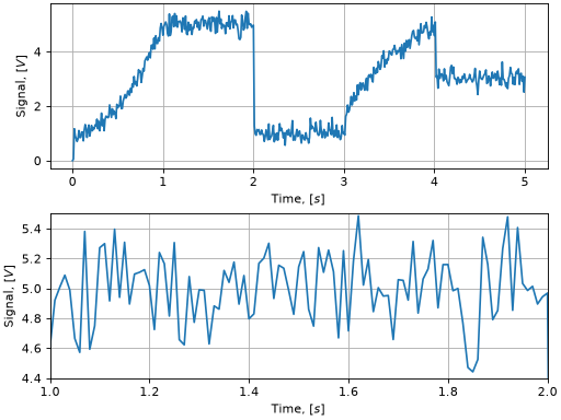
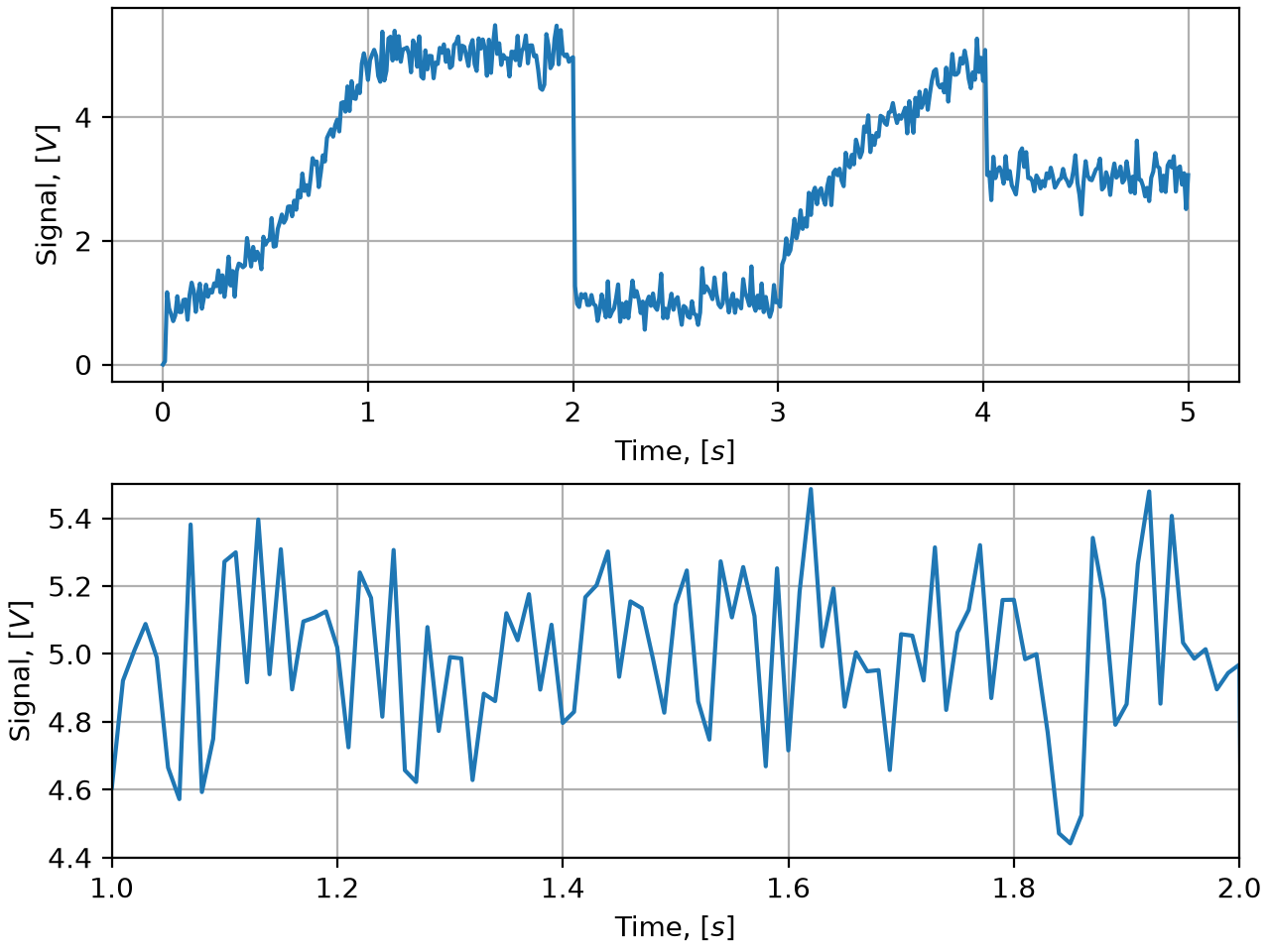
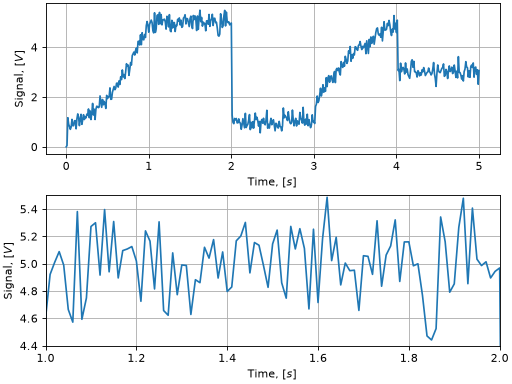
Pressure sensor electrical signal historical values

When considering the time interval from \([1 − 2] [s]\), the influence of measurement errors with the standard deviation \(0.2 [V]\) is observed.

For the purposes of this section, the pressure sensor demonstration model is implemented in the form of a basic diagram without detailed consideration of the pressure sensor features.

In order to learn the practical implementation the Kalman filter on the REPEAT VISION platform, you need to configure the Kalman filter elements to process the pressure sensor measurements.

3.  Description of the mathematical model

To implement the Kalman filter, it is required to prepare the matrices of equations (1) and (2). This section describes the steps required to prepare the required matrices.

To describe the historical values of the electrical signal, the system state vector should include:

1. Voltage value \(\mathbf х\),

2. First derivative of signal value in time \(\mathbf v\)(value change rate)

The value of the current state of the system at the time \(t_k\) is connected with the previous state of the system at time \(t_{k-1}\) by the relationship (3).

(3)\[\begin{split}\left\{ \begin{aligned} \mathbf x_k &= \mathbf x_{k-1} + \mathbf v \Delta t \\ \mathbf v &= \mathbf v \end{aligned} \right. \end{split}\]

3.1.  System state transition matrix

In the first and main step of implementing the Kalman filter, to solve the above problem, it is necessary to prepare a transitional state matrix of the system \(\mathbf F\) for the equation (1).

The transitional state matrix based on the equation (3) is as follows.

(4)\[\begin{split}\mathbf{F} &= \begin{bmatrix} 1 & \Delta t \\ 0 & 1\end{bmatrix}\end{split}\]

As a result of the first step, the equation (1) will be the following.

\[\begin{split}\mathbf x_k &= \mathbf{Fx}_{k-1} = \begin{bmatrix} 1 & \Delta t \\ 0 & 1\end{bmatrix} \begin{bmatrix}x_{k-1} \\ v\end{bmatrix}\end{split}\]

3.2.  Normal random noise of the system

In the second step, it is required to describe \(\mathbf w_k\) the normal random noise of the system for the [measurement step(#problem_formulation) \(\Delta t = 0.01 [s]\). The \(\mathbf Q\) matrix of normal random discrete noise of the system is set by the equation (5).

(5)\[\begin{split}\begin{aligned} \mathbf w_k &\sim N(0, \mathbf Q) \\ \mathbf Q &= \begin{bmatrix} \frac{\Delta t^4}{4} & \frac{\Delta t^3}{2} \\ \frac{\Delta t^3}{2} & \Delta t^2\end{bmatrix} \sigma_{w}^2 \end{aligned}\end{split}\]

In the equation (5) \(N(0, \mathbf Q)\) - is the normal distribution of \(\mathbf Q\) with an expected value of 0; \(\sigma_{w}\) - is the standard deviation of the random noise of the system.

As a result of the second step, the equation (1) will be the following.

\[\begin{split}\mathbf x_k &= \mathbf{Fx}_{k-1} + \mathbf{w_k} \\ &= \begin{bmatrix} 1 & \Delta t \\ 0 & 1\end{bmatrix} \begin{bmatrix}x_{k-1} \\ v\end{bmatrix} + \begin{bmatrix} \frac{\Delta t^4}{4} & \frac{\Delta t^3}{2} \\ \frac{\Delta t^3}{2} & \Delta t^2\end{bmatrix} \sigma_{w}^2\end{split}\]

3.3.  Control matrix

As part of setting the current task, it is not required to describe the control matrix \(\mathbf B_k\), since the system does not imply control actions.

3.4.  Measurement matrix

In the third step, it is required to form an \(\mathbf H_k\) measurement matrix.

In accordance with the problem statement, only the value of the electrical voltage signal \(\mathbf х\) is measured, the rate of change of the signal \(\mathbf v\) is not measured ,the refore the measurement matrix (6).

(6)\[\mathbf H = \begin{bmatrix}1 & 0 \end{bmatrix}\]

3.5.  Normal random measurement noise

In the fourth step, the description of the \(\mathbf v_k\) normal random measurement noise will be required.

In the matrix of normal random noise, dispersions of random measurement values are indicated. For a previously prepared measurement matrix, (6)the normal random measurement noise is the following: (7).

(7)\[\begin{split}\begin{aligned} \mathbf v_k &\sim N(0,\mathbf R) \\ \mathbf R &= \begin{bmatrix}0.2^2 \end{bmatrix} \end{aligned} \end{split}\]

In the equation, (7) \(N(0, \mathbf R)\) - is the normal distribution of \(\mathbf R\) with an expected value of of 0. In the matrix \(\mathbf R\) \(0.2 [V]\) - standard deviation of the random measurement value.

After the formal description of the required Kalman filter matrices, it is necessary to implement the algorithm on the REPEAT VISION platform.

4.  Implementation of Kalman filter on REPEAT VISION platform

In accordance with the equation, the Kalman filter (1) algorithm for assessing the current state of the system requires measurements of the previous state of the system.

To implement the Kalman filter on the REPEAT VISION platform, usage of the block Jython is required. The block allows to describe the algorithm in Python using the Apache Commons Math library, which contains a ready-made execution of the Kalman filter.[2]

4.1.  Review of the demo project in the REPEAT VISION application software

The REPEAT VISION application’s demo projects set contains an example of using the Kalman filter to evaluate measurement results. Next, we will analyze this example, which will help us describe all the necessary steps for implementing a Kalman filter on the REPEAT VISION platform.

In the REPEAT VISION application software add the [DEMO] Kalman filter for measurement results evaluation from the folder Demo projects and open it for later review.

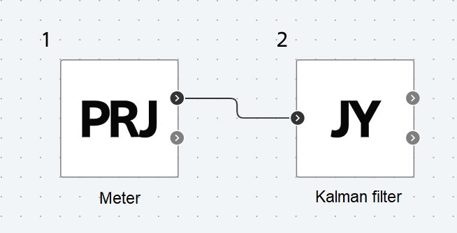
Project with an example of using the Kalman filter to evaluate measurement results

The project contains two blocks (Meter and Kalman filter) and associated global variables that simplify the process of setting the required block parameters.

Sensor block is designed for generation of electrical signal historical values in accordance with the diagram above. Electrical signal values are generated at output signal port of signal block. This block also generates voltage values ​​at the output port theoretical_value that do not contain measurement errors, for the convenience of further analysis of the simulation results.

The project contains a set global variables according to the table below.

Variable name	Variable value	Purpose
SENSOR_MEASURE_ERROR	0.2	Standard deviation of the measurement random value for the Jython block.
PROCESS_NOISE	30	Standard deviation of the random noise of the \(\sigma_{w}\) system for the equation (5)

Next, we will proceed to an overview of the Kalman filter algorithm in the Jython block (№2 in the figure above).

4.2.  Overview of program code in Jython block

For review the Kalman filter algorithm, you need to press the Edit block code in properties of block Jython.

Added in version 3.0.0: The Jython block now supports dividing the block’s program into three stages of the modeling process.

1. Initialization - the code in this stage is executed to prepare for the calculation process. At this stage, it is necessary to import required libraries and create objects whose state needs to be preserved between integration steps during the calculation;

2. Calculation Code - The code in this stage is executed at each integration step from start to stop. This stage runs after initialization;

3. Completion - the code in this stage is executed when the calculation stops.

Next, in the block’s code editor Jython, switch to the Initialization tab to analyze the preparation and setup code for the Kalman filter algorithm.

At the initialization stage, the necessary classes are imported from the Apache Commons Math library.

"""
Jython скрипт предназначен для настройки  фильтра Калмана 
на платформе REPEAT VISION с использованием библиотеки Apache Commons Math.

Скрипт должен выполняться на этапе подготовки к процессу выполнения расчёта
"""
from org.apache.commons.math3.linear import Array2DRowRealMatrix, ArrayRealVector
from org.apache.commons.math3.filter import DefaultProcessModel, DefaultMeasurementModel
from org.apache.commons.math3.filter import KalmanFilter

• Lines 1, 6. Brief description of the purpose and features of the program implementation;

• Line 7. Import the required data structures from the linear algebra module of Apache Commons Math the library. The Array2DRowRealMatrix matrix and ArrayRealVector vector of real values will be used later to configure the Kalman filter classes;

• Lines 8, 9. Importing classes to configure Kalman filter. The DefaultProcessModel class allows to customize the Kalman filter matrices in the equation part (1). The DefaultMeasurementModel class allows to customize them in the equation part (2). The KalmanFilter class, based on the tuned matrices, will allow to calculate the dynamic system state based on the Kalman filter algorithm.

Overview of the function for setting up the Kalman filter

The next step in the initialization phase is to consider the function that performs the tuning of the Kalman filter.

def get_kalman_filter(dt, measure_noise_std, process_noise_std):
  """
  Возвращает фильтр Калмана для оценки состояния динамической системы
  на основании измерения значения сигнала.
  Данный фильтр Калмана учитывает первую производной состояния системы.
  Данная реализация фильтра Калмана подходит для описания следующих процессов:

    - Измерение одного параметра физического процесса;   
    - Движение объекта вдоль одного направления координат.

  Parameters
  ----------
  dt : float
    Временной шаг изменения состояния системы.
  measure_noise_std : float
    Стандартное отклонение случайной величины измерений.
  process_noise_std : float
    Стандартное отклонение случайного шума системы.

  Returns
  -------
  kf : KalmanFilter
    Объект фильтра Калмана
  """
  
  trans_m = Array2DRowRealMatrix([
    [1., dt], # x = x_{k-1} + v*dt
    [0, 1.]   # v = v
  ])
  measure_m = Array2DRowRealMatrix([
    [1., 0] #  измерение только значения сигнала
  ])

• Lines 12, 34. Description of the task performed by the get_kalman_filter function, as well as the description of the arguments of the function and the returned result;

• Lines 36, 39. Creation of transition matrix of the system state in accordance with (4);

• Lines 40, 42. Creates a measurement matrix according to(6) (6).

  measure_noise_m = Array2DRowRealMatrix(
    [measure_noise_std**2]
  )
  pocess_noise_m = Array2DRowRealMatrix([
    [dt**4 / 4, dt**3 / 2], 
    [dt**3 / 2, dt**2]
  ]).scalarMultiply(process_noise_std**2)
  initial_values = ArrayRealVector([1., 0])
  initial_error_cov = Array2DRowRealMatrix([
    [1, 1],
    [1, 1]
  ])

• Lines 43, 45. Creation of a matrix of normal random noise of measurements in accordance with (7);

• Lines 46, 49. Creation of a matrix of normal random discrete noise of the system in accordance with (5);

• Line 50. Creation of initial values of signal measurement and signal change rate;

• Lines 51, 54. Creating the initial values for the initialErrorCovariance covariance matrix of the DefaultProcessModel class.

  process_model =  DefaultProcessModel(
    trans_m, # Переходная матрица состояния системы 
    None, # Матрица управления
    pocess_noise_m, # Матрица нормального случайного дискретного шума системы
    initial_values, # Начальные значения измерения сигнала
    initial_error_cov # Начальные значения initialErrorCovariance
  )
  measure_model = DefaultMeasurementModel(
    measure_m, # Матрица измерений
    measure_noise_m # Матрица нормального случайного шума измерений
  )
  kf = KalmanFilter(process_model, measure_model)

  return kf

• Lines 55, 61. An instance of the DefaultProcessModel class is created with the equation matrix settings (1);

• Lines 62, 65. An instance of the DefaultMeasurementModel class is created with the equation matrix settings(2);

• Lines 66, 68. An instance of the KalmanFilter class is created, configured, and returned from the function KalmanFilter.

The function must be used in a Jython block script at the initialization stage to obtain a configured instance of the Kalman filter.

Initialization of Kalman filter

Below is a description of the program code at the initialization stage of the Kalman filter.

dt = 0.01
measure_noise_std = SENSOR_MEASURE_ERROR 
process_noise_std = PROCESS_NOISE

sensor_kf = get_kalman_filter(dt, measure_noise_std, process_noise_std)

• Line 70. The parameter dt of the time step of changing the system state is created in accordance with the problem statement;

Added in version 2.6.0: Jython block user programs have the ability to apply global project variables. An example of using this feature is given in lines 71-72.

• Lines 71, 72. The following parameters are created: standard deviation of the random measurement values, standard deviation of the random noise of the system, and the default value of the previous measurement. Parameter values are assigned from previously created global project variables;

• Line 74. An instance of the KalmanFilter Kalman class is created and configured according to the description of the get_kalman_filter function.

The entire code of the initialization stage program

During the initialization phase, the code below is executed.

"""
Jython cкрипт предназначен для настройки  фильтра Калмана 
на платформе REPEAT VISION с использованием библиотеки Apache Commons Math.

Скрипт должен выполняться на этапе подготовки к процессу выполнения расчёта
"""
from org.apache.commons.math3.linear import Array2DRowRealMatrix, ArrayRealVector
from org.apache.commons.math3.filter import DefaultProcessModel, DefaultMeasurementModel
from org.apache.commons.math3.filter import KalmanFilter

def get_kalman_filter(dt, measure_noise_std, process_noise_std):
  """
  Возвращает фильтр Калмана для оценки состояния динамической системы
  на основании измерения значения сигнала.
  Данный фильтр Калмана учитывает первую производной состояния системы.
  Данная реализация фильтра Калмана подходит для описания следующих процессов:

    - Измерение одного параметра физического процесса;   
    - Движение объекта вдоль одного направления координат.

  Parameters
  ----------
  dt : float
    Временной шаг изменения состояния системы.
  measure_noise_std : float
    Стандартное отклонение случайной величины измерений.
  process_noise_std : float
    Стандартное отклонение случайного шума системы.

  Returns
  -------
  kf : KalmanFilter
    Объект фильтра Калмана
  """
  
  trans_m = Array2DRowRealMatrix([
    [1., dt], # x = x_{k-1} + v*dt
    [0, 1.]   # v = v
  ])
  measure_m = Array2DRowRealMatrix([
    [1., 0] #  измерение только значения сигнала
  ])
  measure_noise_m = Array2DRowRealMatrix(
    [measure_noise_std**2]
  )
  pocess_noise_m = Array2DRowRealMatrix([
    [dt**4 / 4, dt**3 / 2], 
    [dt**3 / 2, dt**2]
  ]).scalarMultiply(process_noise_std**2)
  initial_values = ArrayRealVector([1., 0])
  initial_error_cov = Array2DRowRealMatrix([
    [1, 1],
    [1, 1]
  ])
  process_model =  DefaultProcessModel(
    trans_m, # Переходная матрица состояния системы 
    None, # Матрица управления
    pocess_noise_m, # Матрица нормального случайного дискретного шума системы
    initial_values, # Начальные значения измерения сигнала
    initial_error_cov # Начальные значения initialErrorCovariance
  )
  measure_model = DefaultMeasurementModel(
    measure_m, # Матрица измерений
    measure_noise_m # Матрица нормального случайного шума измерений
  )
  kf = KalmanFilter(process_model, measure_model)

  return kf

dt = 0.01
measure_noise_std = SENSOR_MEASURE_ERROR 
process_noise_std = PROCESS_NOISE

sensor_kf = get_kalman_filter(dt, measure_noise_std, process_noise_std)

The sensor_kf object, an instance of the KalmanFilter class, will maintain its state between integration steps during the calculation, the code for which is generated in the next step, discussed in the section below.

Modeling code overview

Next, in the text editor of the Jython block code, you need to go to the Modeling code tab to analyze the program that is executed at each integration step from the initial time of the simulation until the calculation is stopped.

Important

Objects created within the modeling code do not retain their state after the integration step is completed.

If your objects need to maintain state between integration steps, they must be created and configured during the initialization phase, and then used in the modeling code.

After initializing all the necessary data, it is necessary to execute the Kalman filter program to estimate the state of the system based on the set of measured values ​​of the system state. The order of work should include:

1. System state evaluation, which is performed by the .predict() method of the KalmanFilter class instance , which is assigned to an object named sensor_kf in the code loop below;

2. Specifying the state of a system that is performed by the .correct() method of an instance of the KalmanFilter class.

After each step of the system state evaluation cycle performance, the values are returned by the .getStateEstimation() method of the KalmanFilter class instance.

"""
Jython cкрипт предназначен для применения фильтра Калмана 
в процессе выполнения расчёта.
"""

current_measure = in_1 
sensor_kf.predict()
before_update = sensor_kf.getStateEstimation()
sensor_kf.correct(
  ArrayRealVector([current_measure])
)
after_update = sensor_kf.getStateEstimation()
out_1 = before_update[0]
out_2 = after_update[0]

After the Kalman filter operation cycle is completed, the results of the system state assessment are generated, which are transmitted to the output ports of the Jython block:

• The signal value is transmitted to the out_1 port;

• The out_2 port receives the signal evaluation value after the system status has been updated based on the current measurement at the \(t_k\) time point.

out_1 = before_update[0]
out_2 = after_update[0]

4.3.  Results of Kalman filter operation on measurement evaluation

Start the calculation project and create a new graph in the Visualization panel.

Add parameters to the graph according to the table below.

Parameter	Description
{bdg-light}`Project [1] - signal	Historical values of the electrical signal of the pressure sensor in accordance with the problem statement.
Project [1] - theoretical_value	Voltage values ​​that do not contain measurement errors
Jython [2] - out_1	Signal evaluation values of Kalman filter from port out_1 of Jython block
Jython [2] - out_2	Signal evaluation values after system state specification from port out_2 of the Jython block

Further, the analysis of the operation of the Kalman filter is required.

At the first analysis stage of the Kalman filter operation, it is required to consider all historical measurement values and their corresponding system state evaluations of the Kalman filter.

(png, hires.png)

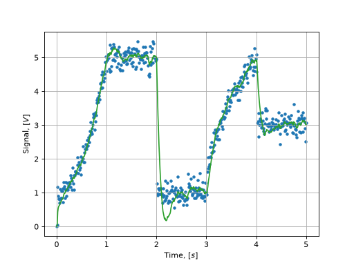
Results of Kalman filter measurements evaluation

The following symbols are used in the graph above.

Lines, labels	Description
Blue tags	Pressure sensor electrical signal historical values
Green line	Evaluation of the state of the system by Kalman filter

Next, it is required to consider the Kalman filter evaluation on the time range \([0.2 - 1] [s]\) with a smooth increase of the electric signal values.

(png, hires.png)

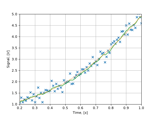
Results of Kalman filter measurements evaluation at time range [0.2 - 1] [s].

The following symbols are used in the graph above.

Lines, labels	Description
Blue tags	Pressure sensor electrical signal historical values
Orange dotted line	Theoretical values
Green line	Evaluation of the state of the system by Kalman filter followed by the specification of the state

In the range {math}`[0.2 − 1] [s], the proximity of the evaluation values of the Kalman filter to the signal measurements is observed, particularly after updating the state of the system (green line).

At the next stage, it is necessary to consider the system state evaluation by the Kalman filter in the range \([0.9 - 1.4] [s]\), when the measurements move from smoothly increasing values to constant values (including the standard deviation of random variables) of the measurements.

(png, hires.png)

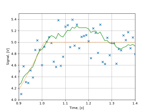
Results of Kalman filter measurements evaluation at the [0.9 - 1.4] [s] time range.

It should be noted that the Kalman filter requires a certain amount of time to be able to estimate the subsequent state with constant values of measurements.

Hint

If a more accurate evaluation of the system state is required in this area, then the control matrix \(\mathbf B_k\), must be considered in the Kalman filter configuration, and the control vector \(\mathbf u_k\) must be included in the Kalman filter cycle.

The graph below also clearly shows that at the time point \(t = 3.1 [s]\), the state of the system was evaluated with a constant value of the signal, the measurement shows the increase of the signal, which was used for state specification of the system by the Kalman filter.

(png, hires.png)

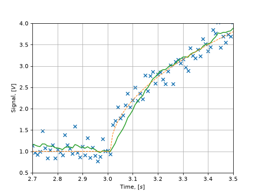
Results of Kalman filter measurements evaluation at the time range [2.7 - 3.5] [s].

Tip

To adapt the Kalman filter to current historical data of measurement results, it is recommended to vary the standard deviation of the random noise of the system (PROCESS_NOISE in the set of global variables of the example of using the Kalman filter on the REPEAT VISION platform)

5.  Conclusions

Within the framework of this practical guide, you managed to master the implementation process of the Kalman filter on the REPEAT VISION platform using the Jython block.

Kalman filter:

• on the one hand, a flexible tool for dynamic systems state evaluation based on measurement results, allowing to work with noisy data;

• on the other hand, the engineer shall have an understanding of the physics of the processes occurring in the system and the ability to formally describe the processes in the mathematical apparatus of the Kalman filter.

The REPEAT VISION platform provides engineers with the necessary toolset to implement the Kalman filter and apply it to interdisciplinary models of industry systems.

6.  References

---

[1] (1,2)

Roger Labbe, Kalman and Bayesian Filters in Python.

[2]

Apache Commons Math. Kalman Filter