

Implementation of DC insert and harmonic analysis of electric power system currents#
Electric power systems undergo a steady complication of their structure, which, in turn, creates specific circuit-mode conditions for the transmission of electricity. The technology of direct current insert (DCI) is used to solve a number of problems that arise under such conditions.
When designing DCI and their control systems (CS), a mathematical simulation apparatus is actively used to assess the impact of the implemented item on the operation of the power system in which it will be integrated, and its operating parameters, on the basis of which the necessary decisions are made.
This practical guide provides an overview of the model that contains DCI and {term} CS of its converter part. During the description of the model, the solutions used to create the model will be considered, as well as the results of simulation in the test power system are given (PS). The DCI model is developed on the REPEAT VISION platform and is available in Item 3 of the Projects section of the Demo projects subsection. It should be noted that the user can download this example and edit the specified parameters of the DCI and CS components for their integration into the designed PS of other configurations.
In this practical guide:
Information is provided on what DCI is and the list of problems in power systems solved with it;
A description is given of the implementation of DCI on the REPEAT VISION platform with a description of its components and the CS algorithm by an inverter;
Interpretation of simulation results by means of given oscillograms and harmonic analysis of PS currents is given.
1. DCI#
Direct current insert is a substation that converts AC to DC from the mains using a rectifier and then converts DC to AC of the original or other frequency at the output using an inverter. In PS it is used to solve the following problems [1]:
Connection of two electric networks of the same nominal frequency, but different non-fixed phase shifts;
Connection of electric networks of various frequencies and phases;
Increase of throughput of network components that contain “weak” connections;
Coordination of network operation in case of emergencies and restoration of power supply after elimination of disturbances.
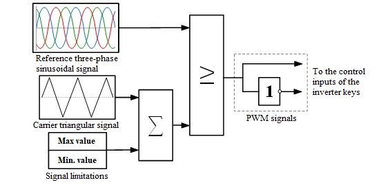
Within the framework of this guide, DCI simulation is considered, connecting two non-synchronously operating PS with frequencies of 60 and 50 [Hz], respectively. The structural diagram of the test PS with DCI and CS of inverter, which is part of it, are shown in Fig. 1 and 2.
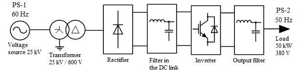
Fig. 1 Block diagram of DCI connecting two non-synchronously operating PS#
2. Implementing DCI on REPEAT VISION platform#
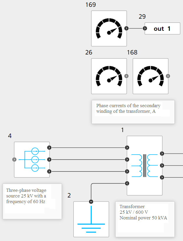
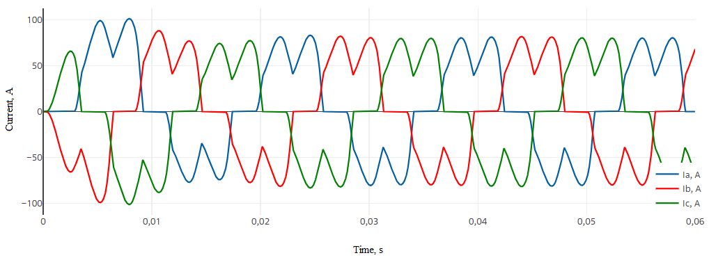
Building PS is done using library blocks Electronics in REPEAT VISION. PS with a frequency of 60 [Hz] (see Fig. 3 below) is given by Three-phase voltage source 25 [kV] block №4, which is connected to Three-phase two windings transformer 25/0.6 [kV] block №1 with Y/D-1 winding connection circuits (phase currents of the secondary winding are fixed by sensors). Fig. 4 shows the oscillograms of the PS-1 current, the non-sinusoidal shape of which indicates its significant harmonic distortion due to the influence of the non-linearity of the converting components of the DC insert. As a result, it is necessary that the implemented DCI and its CS neutralize this drawback and PS-2 load is powered by a current with the required level of sinusoidal. In order to perform harmonic analysis of the current before conversion, the signal from phase A of the secondary winding of the transformer is supplied to Outport block №29 (see Fig. 3 below).
Converter part of DCI is made as serially connected by rectifier and inverter with application of filters on specified sections. In general, the diagram is shown in Fig. 5. Next, a detailed description of the arrangement of this circuit will be given, considering the corresponding simulation results for current and voltage conversion.
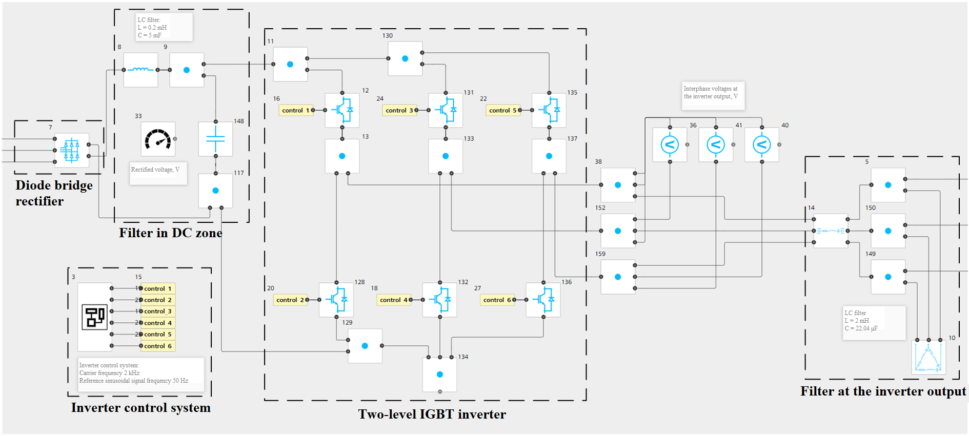
AC voltage coming from PS-1 passes through Three-phase rectifier block №7, which is made by two serially connected three-phase groups of diodes. Rectified DC voltage is supplied to the inductance-capacitance filter consisting of block №8 Inductor and of block №148 Capacitor with parameters of 0.2 [mH] and 5 [mF] to minimize pulsations, which is necessary to eliminate their negative impact on the operation of both the converter and the powered load (Fig. 6, 7).
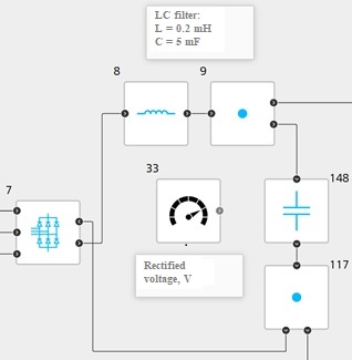
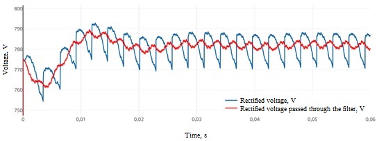
Fig. 7 Rectifier output voltage and its filtering#
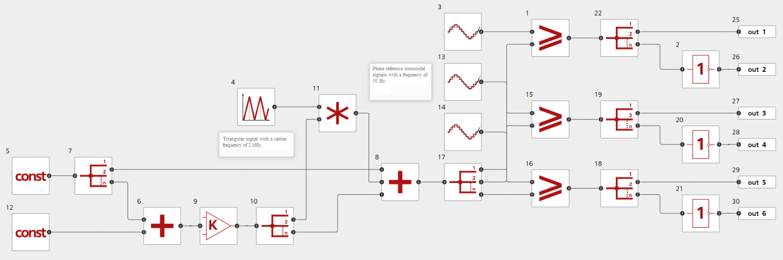
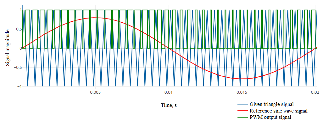
Let’s consider the operation logic of CS of inverter. CS is implemented using Automation library blocks and is shown in Fig. 8. The algorithm implements sinusoidal pulse-width modulation (PWM) at a carrier frequency of 2 [kHz], the principle of which is to compare the reference signals that form a three-phase voltage system of sinusoidal shape blocks №3, №13, №14 Sampled sinusoidal wave, with the specified Triangular signal block №4. Blocks №1 and №12 Constant determines the minimum and maximum values of triangular signal. Each pair of controlled switches of the inverter DCI is associated with its own carrier signal, which determines the switching moments at the points of intersection with the normalized instantaneous value of the specified voltage [2]. Generated PWM signals are transmitted to control inputs via Outport blocks №25-30 to determine the state inverter switches, whereby a pulse sequence of phase voltages is formed. For clarity, the process of generating control pulses for switches corresponding to phase A, implemented by the algorithm, is given in Fig. 9. A change in the carrier frequency of the triangular signal will affect the output signal PWM, which will directly affect the sinusoidal form of the form of the output current PS-2, therefore, when introducing DCI into other models, it is necessary to adjust the value of the carrier frequency depending on the circuit-mode features PS.
The DC link voltage is supplied to a two-level IGBT inverter Fig. 10, which converts the DC voltage into AC voltage with a frequency of 50 [Hz] at the output using the CS described above (its modulated form is shown in Fig. 11). Inverter control keys are represented by Transistor with reverse diode blocks №12, №128, №131, №132, №135 and №136 (transistors get opened under the condition of direct displacement of the collector-emitter junction and the signal PWM equal to 1 through blocks №15, №19, №23, №17, №21 and №25 GO TO with the names “control_1 - control_6”). At the inverter output there is an inductive-capacitive filter made with Three-phase series RLC branch block №14 with inductance of phase 2 [mH] and [Three-phase series RLC delta load](../../../../reference/blocklib/electronics/passiveElements/ElectronicThreePhaseLoadDeltaSeriesConnection/index.md) {bdg-info-line}block №10`, with inter-phase capacity 22.04 [μF]. This filter is necessary to form the required sinusoidal output current (see Fig. 12 below) that powers the load PS-2 with a power of 50 [kW]. Current of phase A of the load is supplied to Outport block №31 named “out_2” for harmonic analysis of current after conversion.
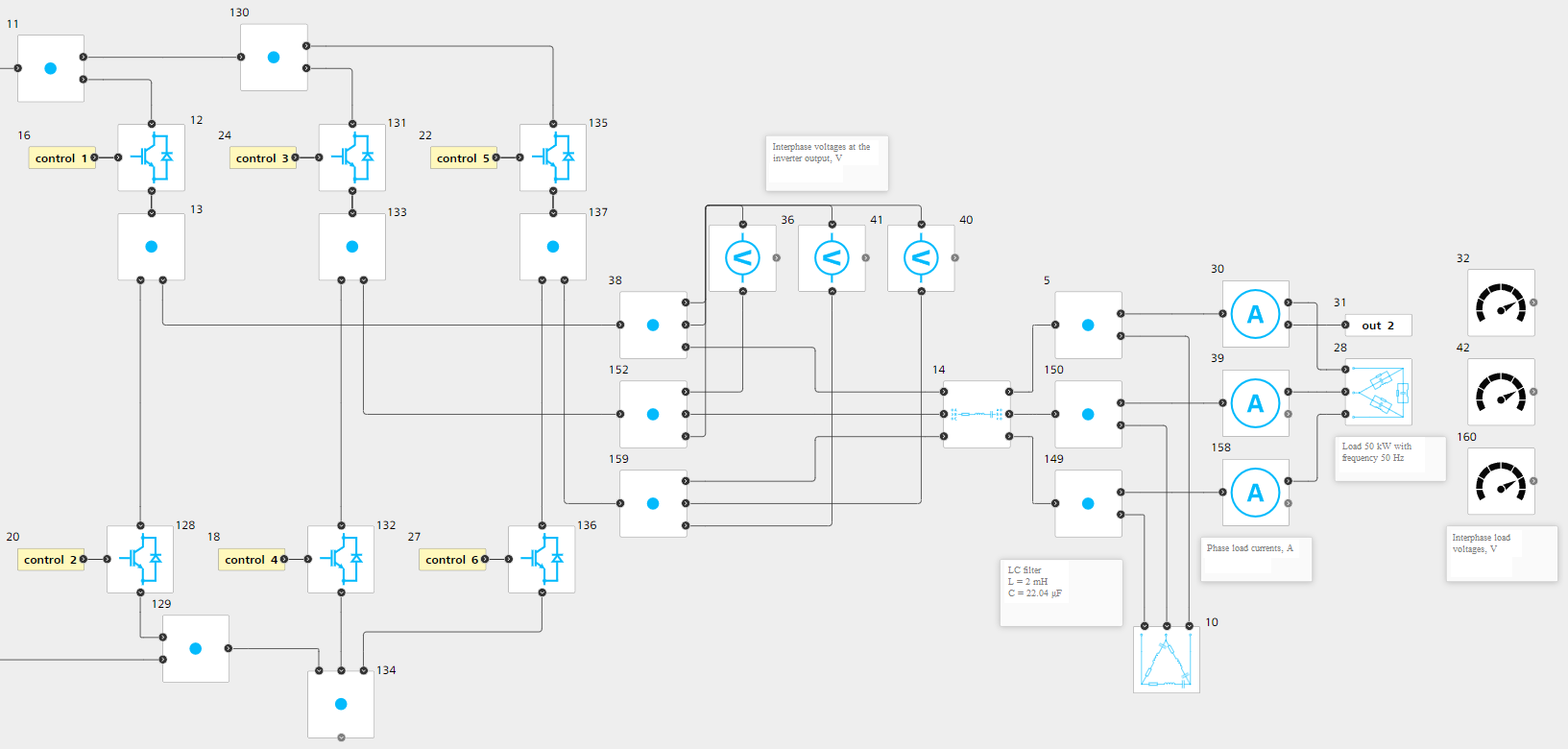
Fig. 10 Inverter DCI, output filter and powered load PS-2 with frequency 50 [Hz]#
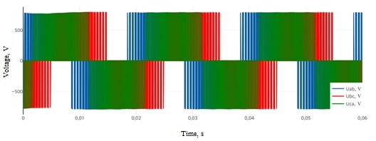
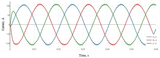
The simulation results correspond to the theoretical idea of voltage conversion by means of power electronics [3], as a result of which it is possible to declare the correctness of this model.
3. Harmonic analysis of power system currents#
In order to assess the effectiveness of the solutions used to ensure the necessary sinusoidality of the output current during the design, a harmonic analysis is carried out, which allows to visually and quantitatively characterize the composition of the harmonics of the currents. In order to implement it, let’s use the built-in tool JupyterLite, with which one can process the simulation results through a fast Fourier transform.
It is important to note that a feature of the program implementation through the used NumPy library is its dependence on the simulation time and sampling rate in the design project. Accordingly, the frequency of the analyzed current (fundamental harmonic) should be a multiple of the unit division of the frequency spectrum calculated by the program. Below is the principle of its calculation, according to which the user needs to manage the respective time parameter settings for each of the analyzed currents from the program code.
Note
For a more detailed description of setting the simulation parameters in JupyterLite for the model in REPEAT VISION, refer to the ExplorationModel class run method
Let’s set phase A current from PS-1 as “AMP1” and phase A current of the load PS-2 as “AMP2”. Below is a description of the code in JupyterLite for calculating the instantaneous values of currents signal_AMP and the formation of arrays of complex numbers transform, which are the harmonic components of currents, with the output of magnitudes amplitude values and phases phase angles.
# Гармонический анализ токов

# Установка пакета repeat для взаимодействия с платформой REPEAT VISION
import piplite
await piplite.install('repeat')

# Импорт необходимых пакетов
import math
import numpy as np
import pandas as pd
import matplotlib.pyplot as plt
import scipy as sc
from scipy.integrate import quad
from repeat import User, Application, TimeInterval

## Настройка взаимодействия с платформой REPEAT VISION
user = User (
	'…'
) # Указывается индивидуальный API ключ пользователя
app = Application (user)
project = … # ID проекта

# Подключение к проекту 'Вставка постоянного тока'
model = app.get_exploration_model(project)
model

## Настройка параметров времени
# По описанному принципу вычислено, что для получения необходимых единичных делений для
# частотных спектров токов применительно к данному демо-проекту требуется задать время расчета
# 0.05 с для тока 60 Гц (меньше модельного времени) и 0.06 с для тока 50 Гц (соответствует модельному времени)
modeling_time_AMP1 = 0.05 # Время моделирования, с (для тока AMP1)
modeling_time_AMP2 = 0.06 # Время моделирования, с (для тока AMP2)
sampling_step = 0.000004 # Шаг дискретизации и интегрирования, с
solver_step = sampling_step * 10**3  # мс

## Расчёт мгновенных значений токов на платформе REPEAT VISION
with model as md:
    md.run(
	pd.Series({'VAL': 1.}),
	modeling_time = modeling_time_AMP2, # секунды
	integration_step = solver_step, # мс
	discretization_step = solver_step, # мс
    )
    # TimeInterval соответствуют modeling_time_ для каждого из токов (в мс)
    signal_AMP1 = md.get_results('AMP1',  TimeInterval(start = 0, end = 50))
    signal_AMP2 = md.get_results('AMP2',  TimeInterval(start = 0, end = 60))

## Анализ Фурье (FFT)
def get_fft(signal, step):
    """
    Рассчитываются основные величины преобразования Фурье
    """
    # Массив комплексных чисел, представляющий из себя гармонические составляющие тока
    transform = np.fft.fft(signal)
    # Частотный спектр тока
    frequencies = np.fft.fftfreq(len(signal), step)
    # Амплитудные значения (magnitudes) и фазные углы (phases) гармонических составляющих (необходимы для расчета по формуле 3)
    magnitudes = np.abs(transform)
    phases = np.angle(transform)

    return frequencies, magnitudes, phases

# Расчет соответствующих величин для AMP1 и AMP2
fft_signal_AMP1 = np.fft.fft(signal_AMP1)
frequencies_AMP1, magnitudes_AMP1, phases_AMP1 = get_fft(signal_AMP1, sampling_step)
frequencies_AMP2, magnitudes_AMP2, phases_AMP2 = get_fft(signal_AMP2, sampling_step)
Normalized frequency spectra of analyzed currents are given in Fig. 13 and 14 (harmonic values are taken as a percentage of the main harmonic of the current). Code for graphic construction of frequency spectra:
### Подготовка графиков нормированных частотных спектров анализируемых токов

# Нормирование выполняется на **максимальное** амплитудное значение magnitudes_AMP1 и magnitudes_AMP2

normalized_amplitudes = [
    100 * magnitudes_AMP1 / magnitudes_AMP1.max(),
    100 * magnitudes_AMP2 / magnitudes_AMP2.max(),
]
frequencies = [frequencies_AMP1, frequencies_AMP2]
signals = [signal_AMP1, signal_AMP2]
xlim_values = [[(0, modeling_time_AMP1), (0, 1400)], [(0, modeling_time_AMP2), (0, 1400)]]

for i in range(2):
    plt.figure(figsize=(12, 4))

    plt.subplot(1, 2, 1)
    plt.plot(
	signals[i].index / 1e3, # перевод из мс в с
	signals[i]
    )
    plt.xlabel('Время, с', fontsize = 11)
    plt.ylabel ('Ток, А', fontsize = 11)
    plt.grid(True)
    plt.xlim(xlim_values[i][0])

    plt.subplot(1, 2, 2)
    plt.vlines(frequencies[i], 0, normalized_amplitudes[i])
    plt.xlabel('Частота, Гц', fontsize = 11)
    plt.ylabel('Амплитуда, %', fontsize = 11)
    plt.grid(True)
    plt.xlim(xlim_values[i][1])

plt.show()
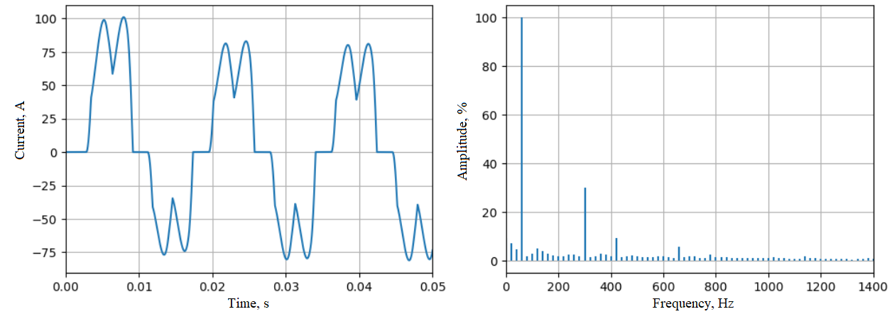
Fig. 13 Phase A current from PS-1 (AMP1) and its normalized frequency spectrum#
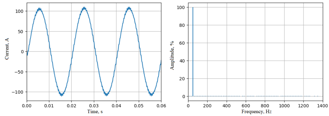
Fig. 14 Load phase A current PS-2 (AMP2) and its normalized frequency spectrum#
From the obtained normalized frequency current spectrum of PS-1, it can be said about the availability of higher harmonics, the value of which is significant in relation to the fundamental harmonics (60 [Hz]). The frequency spectrum of the output current PS-2 has a clear predominance of the fundamental harmonic (50 [Hz]) relative to others and its signal shape is close to ideal sinusoidal.
The quantitative indicator that characterizes the degree of current harmonic distortions is the total harmonic distortion (THD), which is equal to the ratio in percent of the root of the sum of the squares of the mean square values of all harmonics except for the main one to its mean square value [4] (1) :
Where: \(V_n\) – root mean square value of the nth harmonics; \(V_1\) – root mean square value of the fundamental harmonics.
Harmonics RMS formula (2) :
where:
\(T_n\) – period of the n-th harmonics (3) :
where:
\(C_n\) – n-th harmonics amplitude; \(\omega_n\) – n-th harmonics frequency; \(\phi_n\) – n-th harmonics phase angle.
We accept only positive frequency components, as a result of which the following operation is performed:
# Выведение половины частотного спектра, соответствующей положительным составляющим
def get_half(magnitudes, frequencies, phases):
    assert len(magnitudes) == len(frequencies) == len(phases)
    half = slice(
        1, math.ceil(len(magnitudes) / 2)
    )
    return magnitudes[half], frequencies[half], phases[half]
The data obtained is used in the code below, which is necessary for calculating harmonics RMS values and determining total coefficients of harmonic components of currents AMP1 and AMP2.
## Расчёт THD - суммарного коэффициента гармонических составляющих
def calculate_THD(magnitudes, frequencies, phases):
    V_values = []
    iterator = zip(magnitudes, frequencies, phases)
    for mag, freq, phase in iterator:
        def f(t):
            w = 2 * np.pi * freq
            return (mag * np.cos(w * t + phase))**2 # Соответствует формуле 3

        T = 1 / freq
        result, _ = quad(f, 0, T)
        V_values.append(
            (result * freq)**0.5 # Соответствует формуле 2
        )
    V_values.sort()
    V_fundamental = V_values.pop()
    V_others = np.array(V_values)
    THD = np.sqrt(
        (V_others**2).sum()
    ) / V_fundamental * 100 # Соответствует формуле 1

    return THD

THD1 = calculate_THD( * get_half(
    magnitudes_AMP1,
    frequencies_AMP1,
    phases_AMP1
))
print("Суммарный коэффициент гармонических составляющих:", f"{THD1 = } %")

THD2 = calculate_THD( * get_half(
    magnitudes_AMP2,
    frequencies_AMP2,
    phases_AMP2
))
print("Суммарный коэффициент гармонических составляющих:", f"{THD2 = } %")
Based on the calculation results, we have:
For phase A current from PS-1 (AMP1) – THD = 35.62 [%];
For load phase A current PS-2 (AMP2) - THD = 2.55 [%].
The obtained values of the harmonic component coefficients indicate a low harmonic distortion of current PS-2 relative to the current PS-1 and the effectiveness of the measures taken. A clear predominance of the fundamental harmonic is achieved due to the action of PWM and the inductive-capacitive filter at the inverter output, which allows ensuring the necessary sinusoidality of current in PS-2.
4. Conclusions#
The use of DCT is necessary to solve a number of problems characteristic of complex structures of modern electric power systems. This manual described the implemented model DCT in the test PS and CS of its converter part. The simulation results demonstrate the correct operation of the model and the effectiveness of the decisions made;
Within the framework of this manual, it was possible to study the basic concepts of converting current from one type to another by means of power electronics that are part of DCT, as well as integrate its model for connecting non-synchronously operating PS. Using the JupyterLite built-in laptop code will allow harmonic analysis of currents and calculate the total harmonic coefficient for the design of means to ensure sinusoidal currents PS.