

Maximizing gas production rate in the gas well cluster collection system#
The operational need to control the parameters of the well product collection system (WCS), if there is a digital process model, is due to the need to solve the following tasks:
Calculation of WCS parameters for compliance with the technical design of hydrocarbon (HC) field development;
Ensuring maximum HC production during the peak period (winter, demand) and minimum production (summer, demand);
Ensuring optimal parameters of WCS operation at:
Unplanned shutdown of one or several wells;
Well operation modes that do not correspond to the design ones;
Determination of WCS parameters when changing the input parameters of the gas and condensate treatment system.
This practical guide addresses the problem of maximizing the flow (production rate) of a cluster gas collection system containing two gas wells. The simplified collection system comprises several sections of pipelines and 2 nozzles, in which it is necessary to determine the diameters of their holes.
Solving this optimization problem will allow maximizing gas production rate and will help to avoid the occurrence of flows in unspecified directions in the collection system.
1. Prepare gas gathering system model on REPEAT VISION platform#
In the REPEAT VISION application, create a new project called, for example, Gas collection system.
During the preparation of the project on the REPEAT VISION platform, the creation of a model of a gas well cluster (GWC) gas collection system will be demonstrated, shown in the figure below.
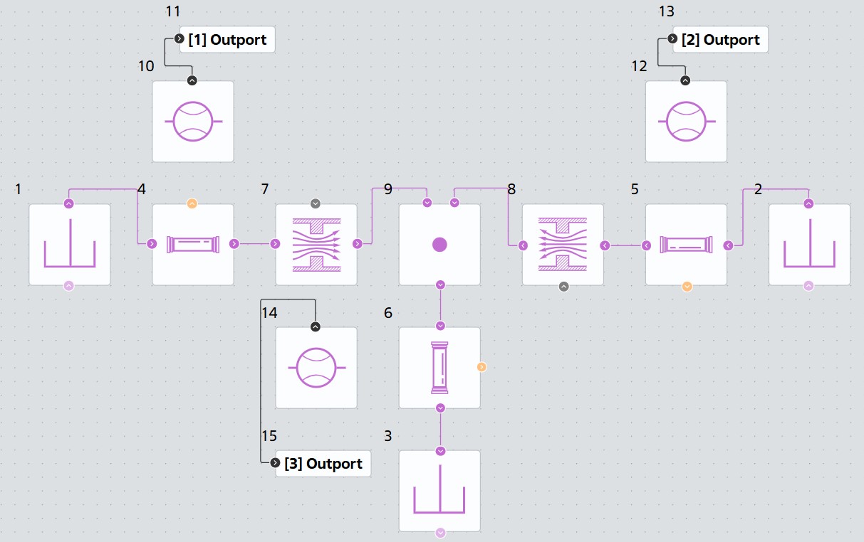
The design of the cluster gas collection system of two gas wells#
A library of Pneumatics blocks of the REPEAT VISION platform is used to create a model of the gas collection system.
The following designations are used in the gas collection system model: the left and right loops are the inlet sections of the pipelines and the lower pipeline is the outlet section of the pipeline system.
Important
It should be noted that with a significant difference in pressure at the wellheads, it is possible to form a reverse flow when gas moves not only from the head of one well into the header, but also compresses another well, reducing the total gas production rate at the GWC.
In order to prevent such situations, nozzles are used on the pipeline loops of the GWC.
1.1. Collection system model creation procedure#
The new Gas collection system project shall use the model settings shown in the figure below.
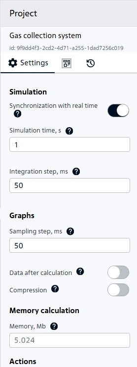
Project settings#
Let’s start creating a model of the gas collection system by adding three blocks Reservoir (P) with different pressures (blocks №1, 2, 3).
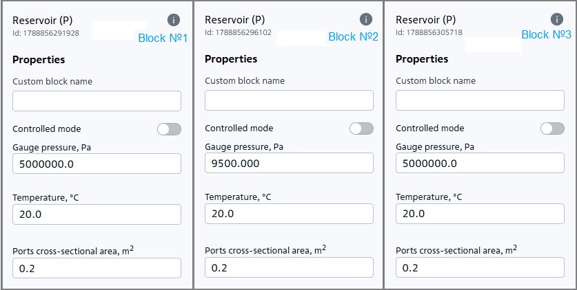
Tanks with different pressures#
Arrange the tanks as follows:
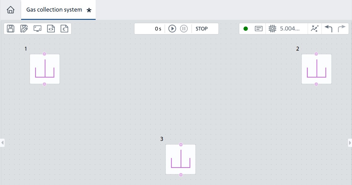
Location of tanks#
The first two tanks designed to set wellhead pressure will be considered as inlet and will be designated as left and right (in the code, respectively, we will add left and right to the variables denoting the parameters of these tanks).
The third tank designed to set the pressure in the header is considered outlet (in the code we will designate it as total).
Connect three identical Pipe (P) (blocks №4, 5, 6) to them with the following parameters.
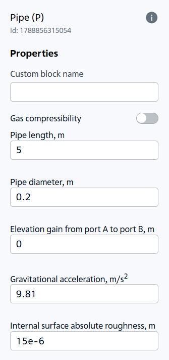
Pipeline section parameters#
Position the pipeline sections as follows:
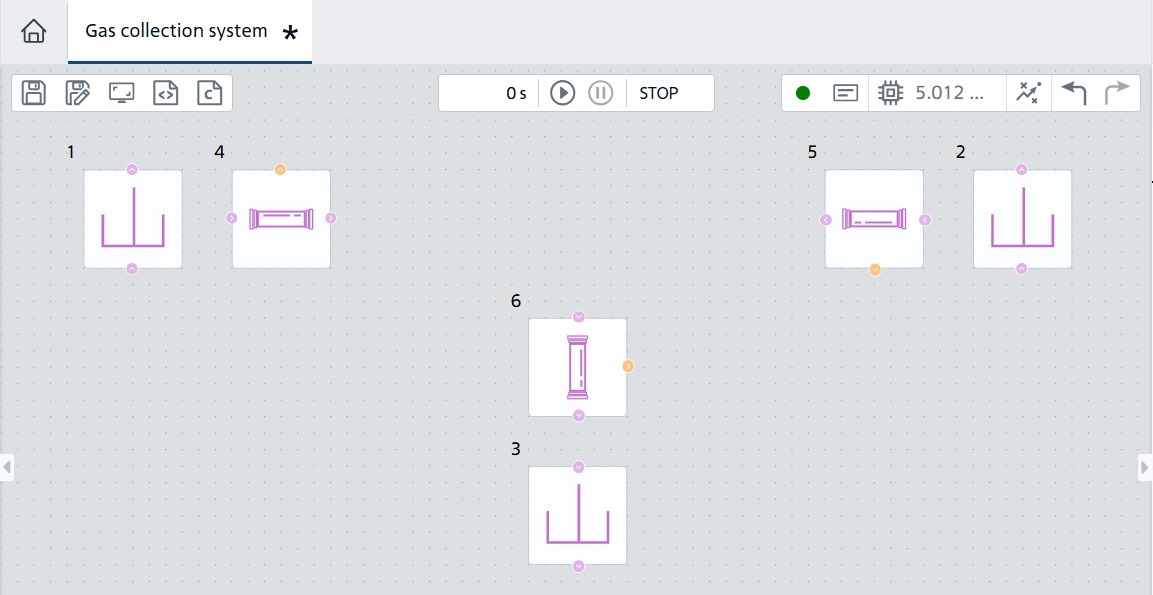
Location of pipeline sections#
In order to subsequently change the cross-sectional area of the holes as part of the optimization problem, create two global variables given in the table below.
Variable name |
Variable value |
Purpose |
|---|---|---|
area_left |
0.02 |
Cross-sectional area of the hole in the left inlet channel of the tee |
area_right |
0.02 |
Cross-sectional area of the hole in the right inlet channel of the tee |
Connect the Orifice (P) blocks (blocks №7, 8) to two of the three pipeline sections. Set Orifice type to Constant. Let’s set the area outside the hole equal to the area of the pipe section in terms of the diameter specified for it and indicate the names of the created variables as the area of the hole section.
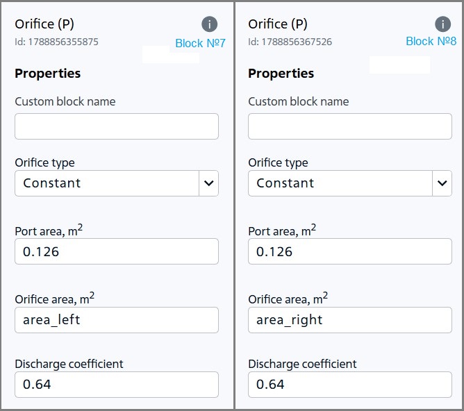
Hole parameters#
Place the holes as follows:
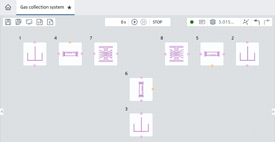
Location of holes#
Let’s close all created components to Node (P) (block №9) with two inputs and one output to the area without a hole. Let’s connect all the created units by turning some of them over:
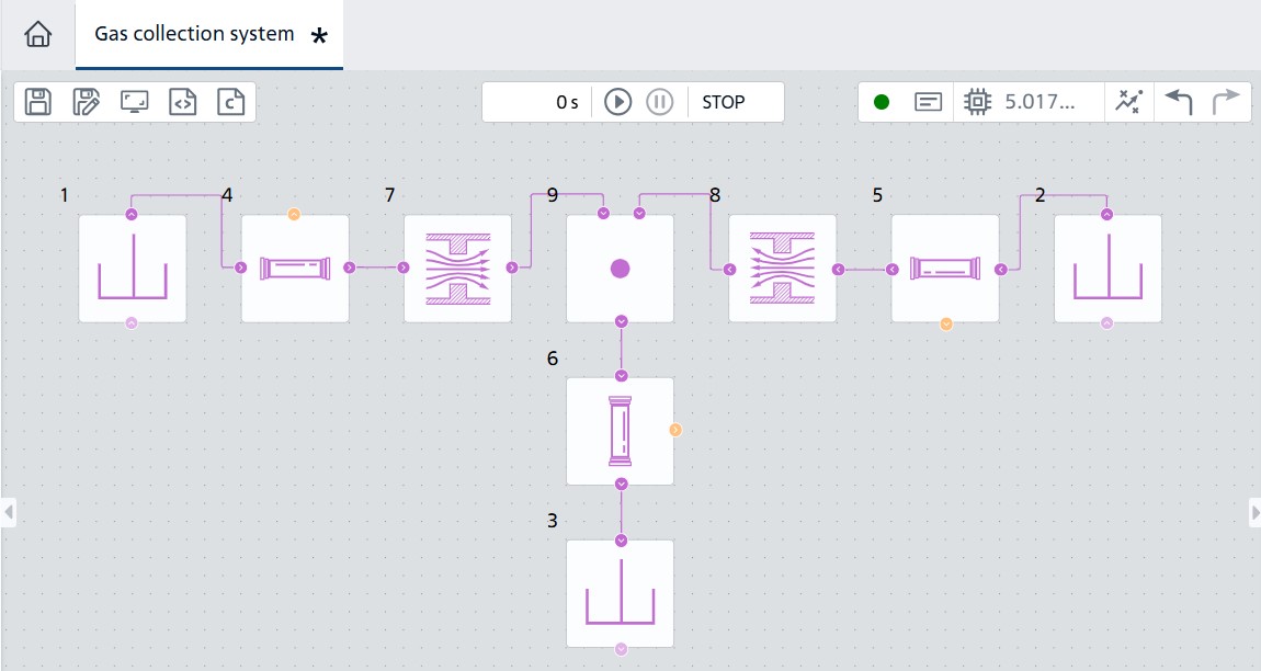
Node connection#
In order to obtain the results of calculation of gas flows in different sections of the pipelines, let’s add Flow Rate Sensor (P) (blocks №10, 12, 14) to each section of the pipeline.
The flow rate sensors shall be connected to the Outport blocks (blocks №11, 13, 15) for further connection of the optimizer to the collection system model.
For example, for the left branch, block №4 Pipe (P) is the related block for the flow rate sensor and the outlet port (block №11) has a user massflow_left name.
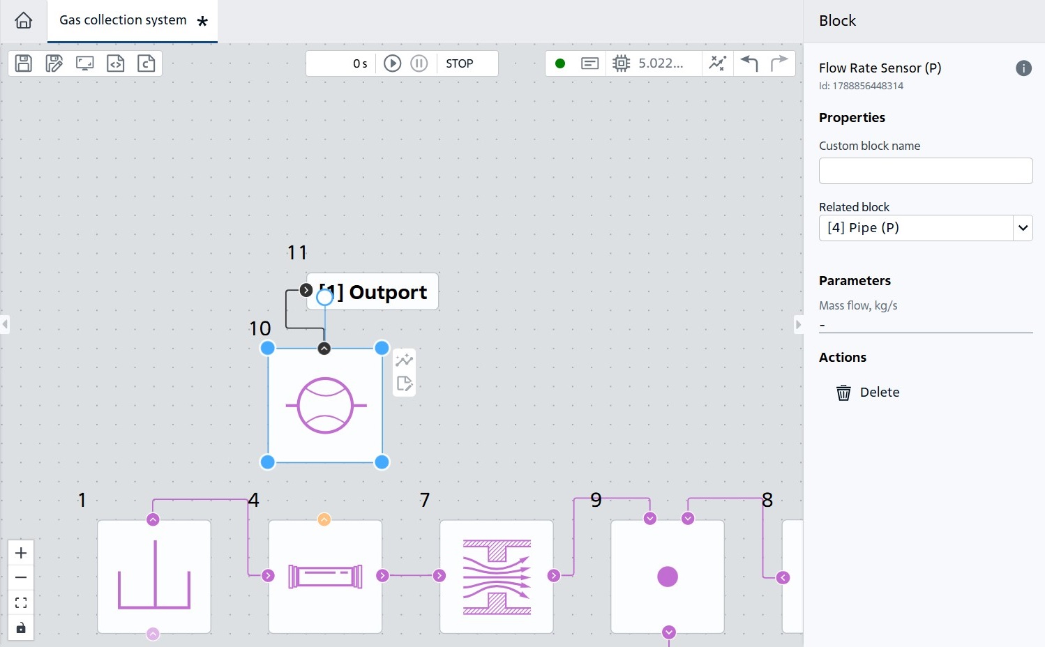
Connection of flow rate sensor and output port#
By analogy, let’s add Flow Rate Sensor (P) and Outport to the rest of the pipeline sections, specify massflow_right and massflow_total, respectively, as a custom name. As a result, we get the following scheme:
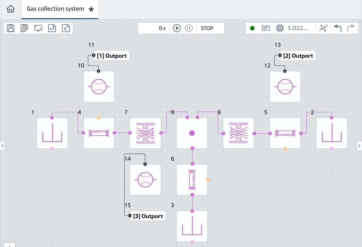
Connection of flow rate sensors and output ports#
Let’s try to calculate:
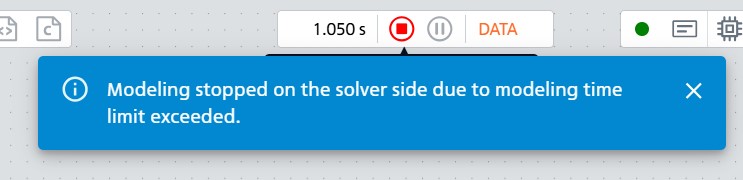
Calculation start#
As you can see, the reverse flow is fixed in the left branch of the tee, which means that the current through the lower branch is not maximum.
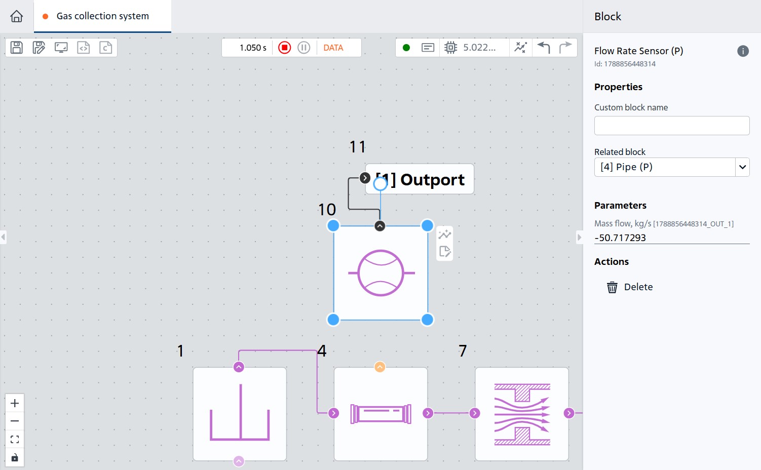
Flow rate sensor indications (block №10)#
Startup results table
Flow rate sensor |
Mass flow rate, kg/s |
|---|---|
Left |
-50.707848 |
Right |
288.25247 |
Lower |
237.54462 |
Let’s optimize the dimensions of the holes to maximize the flow through the lower branch of the tee:
2. Solving an optimization problem using JupyterLite laptop#
Let’s start the JupyterLite development environment by going to the Tools tab by selecting Notebook. In the interface that opens, let’s create a notebook for Python by clicking on the Python (Pyodide) button in Launcher.
In the file that opens, create a cell with a code. Install the necessary libraries:
import piplite
await piplite.install('repeat')
Now import all the necessary libraries. Let’s note right away that we will use the differential evolution algorithm, its implementation from the scipy library.
import pandas as pd
import numpy as np
import repeat as rp
from scipy.optimize import differential_evolution
Let’s connect to the required project using your token and the id of the previously created project with the task set.
user = rp.User(token = YOUR_TOKEN)
app = rp.Application(user)
project = PROJECT_ID
t_interval = rp.TimeInterval(start = 1, end = 1000)
model = app.get_exploration_model(project, t_interval)
Considering that for some parameters the calculation may not be real and will issue an error, add processing of such cases using the try... except structure.
def calculate_massflows(diameter_left: float,
                        diameter_right: float,
                        model) -> dict:
    """
    Вычисляет массовые потоки на основании заданных диаметров.

    Parameters
    ----------
    diameter_left : float
        Диаметр отверстия в левом канале тройника.
    diameter_right : float
        Диаметр отверстия в правом канале тройника.

    Returns
    -------
    results : dict
        Словарь с величинами потоков в соответствующих каналах тройника.

    """

    area_left = np.pi * (diameter_left / 2) ** 2
    area_right = np.pi * (diameter_right / 2) ** 2

    variables = pd.Series({'area_left': area_left,
                           'area_right': area_right},
                          dtype=float)

    try:
        with model as md:
            md.run(variables)
            massflow_left = md.get_results('massflow_left').iloc[-1]
            massflow_right = md.get_results('massflow_right').iloc[-1]
            massflow_total = md.get_results('massflow_total').iloc[-1]

        results = {
            'massflow_left': massflow_left,
            'massflow_right': massflow_right,
            'massflow_total': massflow_total
        }
    except rp.errors.REPEATSolverError as e:
        print(f"Ошибка: невозможно получить результаты для параметров ({area_left}, {area_right}): {e}")
        results = {
            'massflow_left': -np.inf,
            'massflow_right': -np.inf,
            'massflow_total': -np.inf
        }

    return results['massflow_total']
Let’s set the optimization task for holes radii search and limit the number of iterations by setting the population size.
Important
Note the minus sign before the target function calculate_massflows in the program code below. A minus sign is required by the optimizer to determine the maximum gas flow rate.
Otherwise, the optimizer will solve the problem of minimizing the value of the target function.
Let’s supplement the problem by specifying the boundaries of the values that can take diameters:
bounds = [(0.01, 0.2), (0.01, 0.2)]
Let’s call the optimization method by transferring the calculate_massflows function to it and display the returned parameters. One can read more about what the popsize and maxiter parameters mean here.
result = differential_evolution(
    func = lambda diameters: - calculate_massflows(diameters[0], diameters[1], model
    ),
    bounds = bounds,
    popsize=3,
    maxiter=3
)
optimal_diameters = result.x
max_value = - result.fun
print("Оптимальные параметры:",
    f"diameter_left={optimal_diameters[0]}",
    f"diameter_right={optimal_diameters[1]}",
    sep = "\n")
print(f"Максимальное значение функции: {max_value}")
As a result, the algorithm will find the maximum possible flow and the values of the diameters of the holes at which it is achieved.
Оптимальные параметры:
diameter_left=0.024924022453932757
diameter_right=0.2
Максимальное значение функции: 444.67108
See also
The differential_evolution function of the scipy package is one of the possible optimization algorithms, which can be used in this problem.
Other approaches may also be used, for example:
Bayesian optimization and others.
2.1. Code of the entire program#
import piplite
await piplite.install('repeat')
import pandas as pd
import numpy as np
import repeat as rp
from scipy.optimize import differential_evolution
user = rp.User(token = YOUR_TOKEN)
app = rp.Application(user)
project = PROJECT_ID
t_interval = rp.TimeInterval(start = 1, end = 1000)
model = app.get_exploration_model(project, t_interval)
def calculate_massflows(diameter_left: float,
                        diameter_right: float,
                        model) -> dict:
    """
    Вычисляет массовые потоки на основании заданных диаметров.

    Parameters
    ----------
    diameter_left : float
        Диаметр отверстия в левом канале тройника.
    diameter_right : float
        Диаметр отверстия в правом канале тройника.

    Returns
    -------
    results : dict
        Словарь с величинами потоков в соответствующих каналах тройника.

    """

    area_left = np.pi * (diameter_left / 2) ** 2
    area_right = np.pi * (diameter_right / 2) ** 2

    variables = pd.Series({'area_left': area_left,
                           'area_right': area_right},
                          dtype=float)

    try:
        with model as md:
            md.run(variables)
            massflow_left = md.get_results('massflow_left').iloc[-1]
            massflow_right = md.get_results('massflow_right').iloc[-1]
            massflow_total = md.get_results('massflow_total').iloc[-1]

        results = {
            'massflow_left': massflow_left,
            'massflow_right': massflow_right,
            'massflow_total': massflow_total
        }
    except rp.errors.REPEATSolverError as e:
        print(f"Ошибка: невозможно получить результаты для параметров ({area_left}, {area_right}): {e}")
        results = {
            'massflow_left': -np.inf,
            'massflow_right': -np.inf,
            'massflow_total': -np.inf
        }

    return results['massflow_total']

bounds = [(0.01, 0.2), (0.01, 0.2)]
result = differential_evolution(
    func = lambda diameters: - calculate_massflows(
        diameters[0], diameters[1], model
        ),
    bounds = bounds,
    popsize = 3,
    maxiter = 3
)
optimal_diameters = result.x
max_value = - result.fun
print("Оптимальные параметры:",
    f"diameter_left={optimal_diameters[0]}",
    f"diameter_right={optimal_diameters[1]}",
    sep = "\n")
print(f"Максимальное значение функции: {max_value}")
# Оптимальные параметры:
# diameter_left=0.024924
# diameter_right=0.2
# Максимальное значение функции: 444.67108
3. Conclusion#
As a result of following this practical guide, you learned how to use parametric optimization together with the gas collection system model on the REPEAT VISION platform.
The differential evolution algorithm used made it possible to determine the optimal hole sizes that ensure maximum flow through the outlet section of the pipeline.
The results obtained confirm the effectiveness of the approach for solving engineering optimization problems that allow both designing pipeline systems and effectively supporting the operation of existing field facilities.