Development of mathematical model for UAV parachute landing

1.  Introduction

 This guide provides an overview of the step-by-step development and verification of a parachute landing model for an unmanned aerial vehicle (UAV) aircraft configuration in REPEAT VISION using the ODE block, Fig. 1:

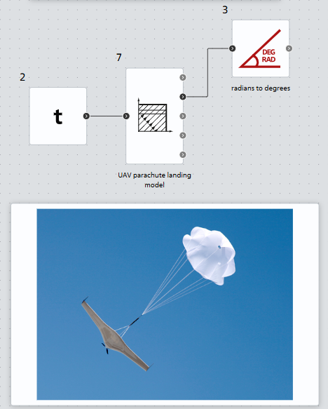
Fig. 1 ODE block in REPEAT VISION

 The mathematical model of the parachute landing of a UAV is based on the monographs on the flight dynamics and control of UAV by V.S. Moiseev [1],[2] (pp. 176–189 in [1]). The model will be verified against the simulation results [1], p. 187.

 Most of the theoretical material will be presented in abbreviated form; for a more detailed description of the mathematical model, please refer to the source [1],[2].

2.  Description of the UAV parachute landing process

 Simulation of the parachute landing process of a UAV allows us to determine its landing point, which will reduce the time it takes to find it for reuse.

 A typical simulated parachute landing system (PLS) of a UAV includes the following elements:

• exhaust parachute (EP);

• main parachute (MP);

• propellant (pyrotechnic) charge (PC(2));

• container for placing EP and MP.

The process of parachute landing of a UAV is divided into the following main stages:

flowchart TD A(__1__ Выброс ВП с помощью МЗ из контейнера СПП после получения соответствующей команды от САУ, выход в поток и наполнение ВП / __1__ Discharge of EP using PC_2 from the PLS container after receiving the corresponding command from ACS, exit to the flow and filling of EP) --> B("`__2__ Вытягивание купола и строп ОП на всю длину / __2__ Pulling the canopy and MP lines to their full length`") B("`__2__ Вытягивание купола и строп ОП на всю длину / __2__ Pulling the canopy and MP lines to their full length`") --> C(__3__ Наполнение купола ОП до площади ограниченной его рифовкой / <br>__3__ Filling the MP dome to the area limited by its reefing) C(__3__ Наполнение купола ОП до площади ограниченной его рифовкой / <br>__3__ Filling the MP dome to the area limited by its reefing) --> D(__4__ Снижение БЛА на зарифованном куполе ОП / <br>__4__ UAV descent on a reefed MP dome) D(__4__ Снижение БЛА на зарифованном куполе ОП / <br>__4__ UAV descent on a reefed MP dome) --> Е("__5__ Разрифовка и наполнение до полной площади купола ОП / <br>__5__ Reefing and filling to the full area of ​​the MP dome") Е("__5__ Разрифовка и наполнение до полной площади купола ОП / <br>__5__ Reefing and filling to the full area of ​​the MP dome") --> F(__6__ Снижение БЛА на полном куполе ОП, приземление и отцепка ОП от БЛА / <br>__6__ UAV descent with the main canopy fully deployed, landing and detachment of the MP from the UAV)

 The simulation of a parachute landing of a UAV is performed under the following assumptions:

• The mass of the charge and container are not taken into account;

• The parachutes used in PLS are inertialess objects;

• All forces acting during the landing process of the UAV are reduced to its center of gravity (CG);

• The movement of the UAV during landing is considered as the movement of its CG in the vertical plane;

• The drag force of a UAV is zero.

3.  Mathematical model of the UAV parachute landing process

 The general equations of motion of the CG UAV during landing have the form (1) :

(1)\[\begin{split}m\cdot \dot{V} = -G ⋅ sin{\theta} - X - X_{п}\\m\cdot V \cdot\dot{\theta}= -G ⋅ cos{\theta}\\\dot{x}=V\cdot cos{\theta}\\\dot{y}=V\cdot sin{\theta} \end{split}\]

where:

 \(X\) - drag force of the UAV;

 \(X_{п} = \Phi_{вп} \cdot \frac{ ho \cdot V_{1}^2}{2\cdot m}\) - parachute drag force;

 \(G\) - UAV gravity: \(G=m \cdot g\)

 \(V\) - landing speed of the UAV;

 \(m\) - mass of the UAV;

 \( heta\) - landing angle of the UAV;

 \(x\) - UAV coordinate along the X coordinate;

 \(y\) - UAV coordinate along the Y coordinate.

 Since there is no data on the drag coefficient of the UAV, \(X\) = 0.

 The initial conditions for this system of differential equations are written as follows (2) :

(2)\[\begin{split}V(t_{0})=V_{пос}\\\theta(t_{0})=\theta_{пос}\\x(t_{0})=x_{пос}\\y(t_{0})=y_{пос}\end{split}\]

 A fairly detailed analysis of the model is given in the monograph [2].

 When modeling the landing of a UAV, the following main stages are considered:

flowchart LR A(__1__ Ввод в действие вытяжного парашюта и вытягивание им основного парашюта / <br>__1__ Deploying the pilot chute and pulling it out of the main parachute) --> B("`__2__ Наполнение основного парашюта / <br>__2__ Inflating the main parachute`") B("`__2__ Наполнение основного парашюта / <br>__2__ Inflating the main parachute`") --> C(__3__ Спуск и приземление БЛА на основном парашюте / <br>__3__ Descent and landing of the UAV using the main parachute)

 As a result, we will reduce the general system to three systems of differential equations with interconnected initial conditions, each of which describes the corresponding stage of the UAV landing.

 The model of the landing process of a UAV at stage 1 has the form (3) :

(3)\[\begin{split}\dot{V_{1}}= -g \cdot sin{\theta_{1}}-\Phi_{вп} \cdot \frac{\rho \cdot V_{1}^2}{2 \cdot m}\\\dot{\theta_{1}}=\frac{-g\cdot cos{\theta_{1}}}{V_{1}}\\\dot{x_{1}}=V_{1}\cdot cos{\theta_{1}}\\\dot{y_{1}}=V_{1}\cdot sin{\theta_{1}}\end{split}\]

where \(\Phi_{vp}\) is the effective resistance of EP.

 The effective drag EP \(\Phi_{vp}\) has the formula (4) :

(4)\[\Phi_{вп} =c_{вп}\cdot F_{вп} \]

where:

 \(c_{п}\) – drag coefficient of the pilot parachute;

 \(F_{п}\) is the area of ​​the pilot parachute dome.

 Initial conditions of the differential equations of the first stage (5) :

(5)\[\begin{split}V_{1}(t_{0})=V_{пос}\\\theta_{1}(t_{0})=\theta_{пос}\\x_{1}(t_{0})=x_{пос}\\y_{1}(t_{0})=y_{пос}\end{split}\]

 In the works [1], [2] in the formula for the angular velocity \(\dot{ heta}\) on the right side of the equation the expression \(G ⋅ cos{ heta}\) is without a minus sign, however, with the initial condition \( heta\) = -180\(^о\) on the right side of the equation a negative derivative will arise, not a positive one, which leads to a decrease in the angle, so a negative factor was added.

 To determine the time \(t_{1}\) of the end of stage 1, we describe the process of pulling ОП with a total mass \(m_{OP}\) and a length \(l_{ОП}\) using the force \(X_{ВП}(t)\) by the second-order differential equation (6) :

(6)\[m_{оп}\cdot \ddot{L}=X_{вп}(t) \]

 The initial conditions for this equation are (7) :

(7)\[\begin{split}L(t_{0})=L_{0}\\\dot{L(t_{0})}=0\end{split}\]

 The following notations are used in the equation:

• \(L = L(t)\) – the length of the part of the MP extended at time \(t\);

• \(m_{OP}= m_{OP}(L)\) – the mass of the part of the MP of length \(L\) extended at this moment in time.

 The mass of the OP, extended by the length \(L\), can be approximately calculated using the formula (8) :

(8)\[m_{ОП}(L)=\frac{\pi \cdot \mu \cdot d^2 \cdot L}{4}\]

where:

\(\mu\) – average density of the material MP;

\(d\) is the average diameter of the MP.

 Using the expression (9) :

(9)\[X_{вп}(t)=\frac{\Phi_{вп} \cdot \rho \cdot V_{1}^2}{2} \]

and the formula for the mass MP DE of the second order (5) can be represented as a system of two first order equations (10) :

(10)\[\begin{split}\dot{L}=l\\\dot{l}=\frac{2 \cdot \Phi_{вп} \cdot \rho \cdot V_{1}^2}{\pi \cdot \mu \cdot d^2 \cdot L}\end{split}\]

with initial conditions (11) :

(11)\[\begin{split}L(t_{0})=L_{0}\\l(t_{0})=0\end{split}\]

 Then the moment of time \(t_{1}\) will be determined from the condition (12) :

(12)\[L(t_{1}) = L_{оп}\]

i.e. when the pilot parachute is extended to the length of the main parachute, opening it.

 Stage 2 of the UAV landing begins with the opening of the main parachute and is described by the following system of differential equations (13) :

(13)\[\begin{split}\dot{V_{2}}= -g \cdot sin{\theta_{2}}-\Phi_{оп}(t,V) \cdot \frac{\rho \cdot V_{2}^2}{2 \cdot m}\\\dot{\theta_{2}}=\frac{-g\cdot cos{\theta_{2}}}{V_{2}}\\\dot{x_{2}}=V_{2} \cdot \cos{\theta_{2}}\\\dot{y_{2}}=V_{2}\cdot sin{\theta_{2}}\end{split}\]

with initial conditions (14) :

(14)\[\begin{split}V_{2}(t_{1})=V_{1}(t_{1})\\\theta_{2}(t_{1})=\theta_{1}(t_{1})\\x_{2}(t_{1})=x_{1}(t_{1})\\y_{2}(t_{1})=y_{1}(t_{1})\end{split}\]

\(\Phi_{оп}(t,V)\) is calculated using the formula (15) :

(15)\[\Phi_{оп}(t,V)= \Phi_{max} \cdot (\frac{t\cdot V}{n\cdot D_{оп}})^k\]

where:

 \(\Phi_{max} = c_{оп} \cdot F_{оп}\) - maximum value of the effective area of ​​the main parachute;

 \(D_{оп}\) - nominal diameter of the parachute;

 \(k, n\) - empirical coefficients.

 Stage 3 is proposed to be described by a model of the type (16) :

(16)\[\begin{split}\dot{V_{3}}= -g \cdot sin{\theta_{3}}-\Phi_{max} \cdot \frac{\rho \cdot V_{3}^2}{2 \cdot m}\\\dot{\theta_{3}}=\frac{-g\cdot cos{\theta_{3}}}{V_{3}}\\\dot{x_{3}}=V_{3}\cdot cos{\theta_{3}}\\\dot{y_{3}}=V_{3}\cdot sin{\theta_{3}}\end{split}\]

with initial conditions (17) :

(17)\[\begin{split}V_{3}(t_{2})=V_{2}(t_{2})\\\theta_{3}(t_{2})=\theta_{2}(t_{2})\\x_{3}(t_{2})=x_{2}(t_{2})\\y_{3}(t_{2})=y_{2}(t_{2})\end{split}\]

 The third stage begins when \(\Phi_{оп}(t,V)=\Phi_{max}\), i.e. when the multiplier \(u=\frac{t \cdot V}{n \cdot D_{оп}}=1\).

4.  Initial data

 Let the UAV, which took off from the ML after completing a flight mission, carry out a parachute landing in the starting CrS, shown in Fig. 2:

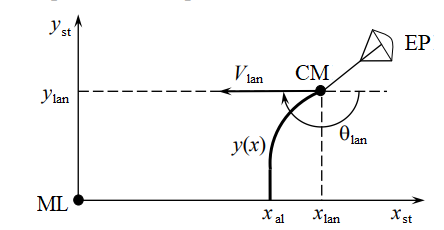
Fig. 2. Parachute landing diagram after a flight mission

 It is believed that the landing of the UAV occurs under normal atmospheric conditions (\(р_{0}\) = 760 mmHg, \( au_{0}\) = +15\(^о\)C) and no wind.

 Initial data:

• Unmanned aerial vehicle:

Characteristic name	Meaning
Landing weight m	300 [kg]

• Exhaust parachute (EP):

Characteristic name	Meaning
Dome area F_{вп}	1.02 [m]
Drag coefficient c_{вп}	0.86

• Main parachute (MP):

Characteristic name	Meaning
Nominal diameter D_{оп}	14 [m]
Dome area F_{оп}	312.4 [m]
Drag coefficient c_{оп}	0.81
Empirical coefficient k	1.6
Empirical coefficient n	2

• Laying the MP:

Characteristic name	Meaning
Length of the elongated OP L_{оп}	31 [m]
Average laying diameter d_{оп}	0.25 [m]
Specific gravity of parachute silk packing μ	1.36

• Other landing parameters:

Characteristic name	Meaning
Air density ρ	1.225 kg/m\(^3\)
Acceleration due to gravity g	9.81 m/s\(^2\)

 Initial conditions of the ODU (Stage 1) (18) :

(18)\[\begin{split}V_{1}(0)=50 \frac{м}{с}\\θ_1 (0)=-180^о\\x_{1}(0)=1000 \hspace{1mm} м\\y_{1}(0)=800\\L(0) = 0.2\hspace{1mm}м\\l = 0\end{split}\]

5.  Development of a model of the UAV landing process in REPEAT VISION

 This section provides an overview of the step-by-step development of the mathematical model under consideration using the ODE block.

Hint

The finished model is also presented in the demo project “[DEMO] UAV parachute landing” in the Demo projects section.

 Block ODE[3] is designed for the numerical solution of systems of ordinary differential equations (ODE) expressed in Cauchy form (with respect to the highest derivative): \(y'' = f(t,y,y')\). Using this block, one can describe a complex dynamic system.

 The entire process of setting up the ODE block consists of 5 key steps:

flowchart LR A(__1__ Очистка шаблона и подготовка рабочего пространства в редакторе кода) --> B("`__2__ Добавление входных/выходных портов и параметров`") B("`__2__ Добавление входных/выходных портов и параметров`") --> C(__3__ Инициализация констант и начальных условий ОДУ) C(__3__ Инициализация констант и начальных условий ОДУ) --> D(__4__ Написание системы ОДУ) D(__4__ Написание системы ОДУ) --> Е("__5__ Настройка и модификация проекта")

 Let’s describe the process of working with the block step by step:

1. When creating and clicking on the ODE block, a script editor for writing the ODE system appears, Fig. 3:

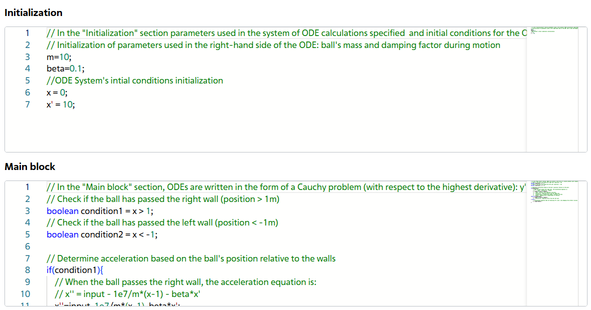
Fig. 3 Code for the template block ODE

 The template block ODE presents a model of a ball bouncing off two walls. To write our model, we will completely clear the sections Initialization, Main block, Additional blocks of code, Fig. 4:

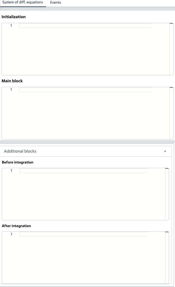
Fig. 4 The code editor for the ODE block after cleaning

next, we will delete the variables located in the right panel (you need to hover over the parameter and click the trash can icon), Fig. 5:

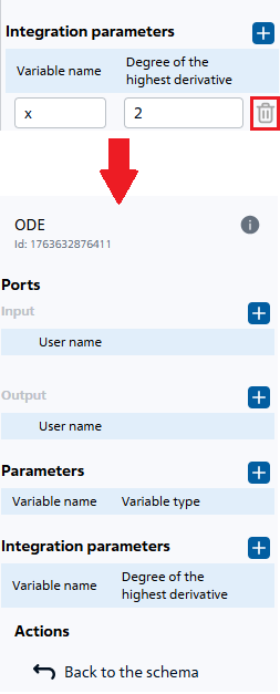
Fig. 5 Removing parameters of the block template ODE

delete in block ODE in the section (1) existing events, by opening the tab of an existing event and clicking on the Delete button (2), Fig. 6:

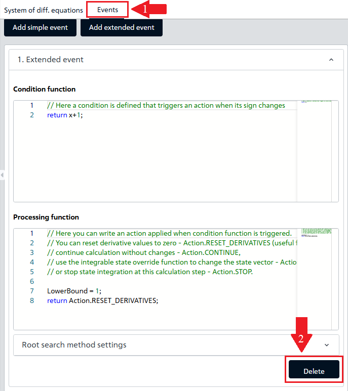
Fig. 6 Deleting events of the ODE block template

 The ODE block is now ready to describe the mathematical model of the dynamic parachute landing system of the UAV.

2. Before writing the ODE system, you need to add the following to the block:

• input and output port parameters;

• parameters involved in the calculation process of ODE;

• integration parameters.

&emspInput port parameters:

1. timer – for removing the simulation time value, participates in the formula \(\Phi_{оп}(t,V)\).

 Output port parameters (see Fig. 7 below):

1. velocity_sensor – to read the value of the landing speed parameter of the UAV;

2. theta_sensor – to read the value of the angle parameter of the UAV, [rad];

3. x_sensor – to read the x-coordinate value, [m];

4. y_sensor – to read the y-coordinate value, [m];

5. L_OP_sensor – for reading the length of the extended part of the MP, [m].

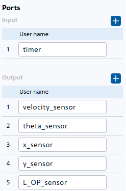
Fig. 7 Required parameters of the ports of the ODE block

 Parameters (see Fig. 8 below):

 m (double) – mass of UAV;

 c_VP (double) – drag coefficient of the pilot parachute;

 f_VP (double) – area of ​​the pilot parachute dome;

 ro (double) – air density;

 mu (double) – specific gravity of parachute silk packing;

 k (double) – empirical coefficient when calculating \(\Phi_{оп}(t,V)\);

 n (double) – empirical coefficient when calculating \(\Phi_{оп}(t,V)\);

 g (double) – acceleration due to gravity;

 phi_VP (double) – effective resistance EP;

 phi_OP (double) – effective resistance MP;

 u (double) – multiplier when calculating \(\Phi_{op}\);

 gndHit (int) – variable signal upon landing of UAV;

 c_OP (double) – drag coefficient of the main parachute;

 f_OP (double) – area of ​​the main parachute dome;

 D_OP (double) – nominal diameter MP;

 d_OP (double) – average diameter of the laying MP.

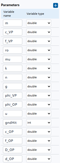
Fig. 8 Required parameters of the ODE block

 Integration parameters:

 velocity is the main parameter for integrating the derivative of the landing acceleration of the UAV \(\dot{V}\), necessary for calculating the speed \(V\);

 theta – parameter for integrating the derivative of the angle \(\dot{ heta}\);

 x – parameter for integrating the derivative of the coordinate \(\dot{x}\);

 y – parameter for integrating the derivative of the coordinate \(\dot{y}\);

 l_OP – parameter for integrating the derivative of the main parachute opening acceleration;

 L_OP – parameter for integrating the derivative of the main parachute opening speed to determine its length \(L_{op}\).

 Integration parameters - the state of the developed system. The ODE block will integrate their derivatives to obtain a numerical solution of the ODE system, Fig. 9:

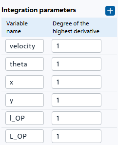
Fig. 9 Integration parameters of the ODE block

3. After adding the parameters, in the code editor we go to the ‘Initialization’ block, where we assign values ​​to the created constant parameters and form the initial conditions of the ODE system, i.e. we set the initial values ​​of the integrated parameters.

m = 300
c_VP = 0.86
f_VP = 1.02
phi_VP = c_VP*f_VP
d_OP = 0.25
D_OP = 14
f_OP = 312.4
c_OP = 0.81
mu = 1.36
k = 1.6
n = 2
g = 9.81
ro = 1.225
gndHit = 0
velocity = 50
theta = -Math.PI
x = 1000
y = 800
L_OP = 0.2
l_OP = 0

• Lines 1-14. Values ​​are assigned to the parameters of the ODE block.

• Lines 15-20. Initialization of the integrated parameters: initial landing speed of the UAV (15), initial landing angle of the UAV (16), initial X-coordinate (17), initial Y-coordinate (18), initial length of the MP (19)

4. Let’s move on to the main part of developing a mathematical model for a UAV landing: we need to describe the ODE system, implementing the \(f(t,y)\) functions in the main block. We’ll begin with the first stage of a UAV landing, when the differential equations describe the operation of the pilot chute:

velocity' = -g*Math.sin(theta) -phi_VP*velocity*velocity*ro/2/m;
theta' = -g*Math.cos(theta)/velocity;
x'=velocity*Math.cos(theta);
y'=velocity*Math.sin(theta);
l_OP'=2*phi_VP*velocity*velocity*ro/(Math.PI*mu*d_OP*d_OP*L_OP);
L_OP'= l_OP;

 The second stage occurs when the main parachute (\(L_{оп} \geq31\)) is fully opened, when the force of resistance to falling is created by MP:

velocity' = -g*Math.sin(theta) - phi_OP*velocity*velocity*ro/2/m ;
theta' = -g*Math.cos(theta)/velocity;
x'=velocity*Math.cos(theta);
y'=velocity*Math.sin(theta);
l_OP'= 0;
L_OP'= 0;

 The ODE block supports the operation of if-else conditional operators, let’s use this function to write a dynamic system. The differential equations for the angle and coordinates remain unchanged and can be moved to the common code area. The code in the main block will look like this:

if(L_OP_sensor<31){
velocity' = -g*Math.sin(theta) -phi_VP*velocity*velocity*ro/2/m ;
l_OP'=2*phi_VP*velocity*velocity*ro/(Math.PI*mu*d_OP*d_OP*L_OP);
L_OP'= l_OP;
} else {
velocity' = -g*Math.sin(theta) - phi_OP*velocity*velocity*ro/2/m ;
l_OP'= 0;
L_OP'= 0;
}
theta' = -g*Math.cos(theta)/velocity;
x'=velocity*Math.cos(theta);
y'=velocity*Math.sin(theta);

• Lines 1-5. Block of code containing the equations for the first stage of landing, when the pilot chute is deployed. This block is executed until the main parachute fully deploys (L_OP_sensor<31);

• Lines 5-9. The code block with the equations for the second landing stage when the main parachute is deployed. The model calculation in this block occurs when the main parachute is fully extended (L_{op} = 31);

• Line 10. Equation for the rate of change of landing angle;

• Line 11. Equation for the rate of change of the X coordinate;

• Line 12. Equation for the rate of change of the Y coordinate.

 However, the code for calculating \(\Phi_{op}\) has not yet been demonstrated, including the transfer of integrated parameter values ​​to the output ports: all this happens in the Advanced tab in the After integration subsection.

velocity_sensor = velocity;
theta_sensor = theta;
x_sensor = x;
y_sensor = y;
L_OP_sensor = L_OP;
if(L_OP>31){
L_OP = 31;
L_OP_sensor = L_OP;
}
u = (timer*velocity)/(n*D_OP);
if(u>1){ 
u = 1;
}
phi_OP = (c_OP*f_OP) * Math.pow(u, k);

• Lines 1-5. Outputting the values ​​of the integrated parameters to the output ports;

• Lines 6-9. Code block to limit the length of MP;

• Line 10. Calculation of the auxiliary function \(u(t,V)\) for calculating the drag force of the main parachute;

• Lines 11-13. Block code for constraint \(u(t,V)\);

• Line 14. Calculation of the drag force of the main parachute.

 Integration parameters can be left standard, i.e.:

• Maximum evaluation count – 10000;

• Integrator type – DormandPrince853;

• Minimum integrator step – 1e-34;

• Maximum integrator step – 1;

• Absolute accuracy – 1e-6;

• Relative accuracy – 1e-6.

 Code in the ODE block editor:

Initialization

m=300;
c_VP = 0.86;
f_VP = 1.02;
phi_VP =c_VP*f_VP;
d_OP = 0.25;
D_OP = 14;
f_OP = 312.4;
c_OP = 0.81;
mu = 1.36;
k = 1.6;
n = 2;
g = 9.81;
ro = 1.225;
gndHit = 0;
L_OP = 0.2;
l_OP = 0; 
velocity = 50;
theta = -Math.PI;
x = 1000;
y = 800;

Main block

if(L_OP_sensor<31){
velocity' = -g*Math.sin(theta) -phi_VP*velocity*velocity*ro/2/m ;
l_OP'=2*phi_VP*velocity*velocity*ro/(Math.PI*mu*d_OP*d_OP*L_OP);
L_OP'= l_OP;
} else {
velocity' = -g*Math.sin(theta) - phi_OP*velocity*velocity*ro/2/m ;
l_OP'= 0;
L_OP'= 0;
}
theta' = -g*Math.cos(theta)/velocity;
x'=velocity*Math.cos(theta);
y'=velocity*Math.sin(theta);

Additional blocks - Before integration

- (Пустое поле)

Additional blocks - After integration

velocity_sensor = velocity;
theta_sensor = theta;
x_sensor = x;
y_sensor = y;
L_OP_sensor = L_OP;
if(L_OP_sensor>31){
L_OP = 31;
L_OP_sensor = L_OP;
}
u = (timer*velocity)/(n*D_OP);
if(u>1) { 
u = 1; 
}
phi_OP = (c_OP*f_OP)*Math.pow(u, k);

5. All that remains is to modify the project itself by adding blocks:

• Simulation time (in section Simulation), which connects to the input port of the ODE block and passes the model calculation time values;

• Angle units conversion (in section Automation, subsection Functions) to convert the landing angle of a UAV from radians to degrees, Fig. 10:

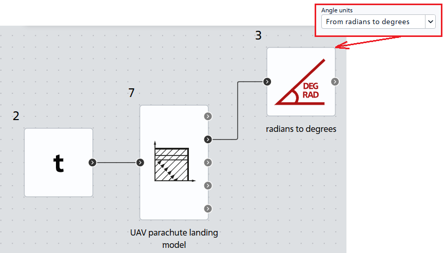
Fig. 10 Project with a mathematical model of UAV landing

 We will select the project simulation time equal to 200 [s], the integration and sampling step is 1 [ms], Fig. 11:

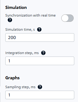
Fig. 11 Project calculation parameters

 The model is ready for calculation. Once the simulation results are obtained, calculation verification can begin.

6.  Simulation results, calculation verification

Table 1 – Comparative analysis of parameters during UAV descent

Stage 1

t, с	Скорость V, м/с Эталон	Скорость V, м/с REPEAT VISION	Скорость V, м/с Абс. погр.	Угол \(\theta\), град Эталон	Угол \(\theta\), град REPEAT VISION	Угол \(\theta\), град Абс. погр.	Координата y, м Эталон	Координата y, м REPEAT VISION	Координата y, м Абс. погр.
0.005	49.976	49.978	0.002	-179.94	-179.944	0.00379	800	800	0
0.011	49.953	49.951	0.002	-179.881	-179.876	0.00472	799.999	799.999	0
0.016	49.929	49.929	0.000	-179.821	-179.820	0.001	799.999	799.999	0
0.021	49.906	49.907	0.001	-179.761	-179.764	0.0027	799.998	799.998	0
0.027	49.882	49.880	0.002	-179.702	-179.696	0.00588	799.997	799.996	0.001
0.064	49.72	49.719	0.001	-179.283	-179.279	0.00448	799.98	799.98	0
0.069	49.698	49.698	0.000	-179.223	-179.222	0.001	799.977	799.977	0
0.074	49.675	49.676	0.001	-179.163	-179.165	0.00244	799.973	799.973	0
0.08	49.652	49.651	0.002	-179.103	-179.098	0.00547	799.969	799.969	0
0.496	19.691	19.693	0.002	-171.352	-171.350	0.00187	799.131	799.13	0.001

Stage 2

t, с	Скорость V, м/с Эталон	Скорость V, м/с REPEAT VISION	Скорость V, м/с Абс. погр.	Угол \(\theta\), град Эталон	Угол \(\theta\), град REPEAT VISION	Угол \(\theta\), град Абс. погр.	Координата y, м Эталон	Координата y, м REPEAT VISION	Координата y, м Абс. погр.
1.329	8.904	8.904	0.000	-136.43	-136.404	0.02587	795.256	795.252	0.0041
2.161	7.25	7.252	0.002	-107.391	-107.390	0.00086	789.634	789.632	0.0017
2.994	6.276	6.276	0.000	-95.2	-95.196	0.00405	784.127	784.123	0.00414
3.826	5.59	5.591	0.001	-91.306	-91.306	0.000275	779.212	779.210	0.0019
4.659	5.097	5.098	0.001	-90.282	-90.282	0.00028	774.773	774.769	0.00426
5.492	4.724	4.724	0.000	-90.053	-90.053	0.00018	770.691	770.684	0.0068
6.324	4.427	4.428	0.001	-90.009	-90.009	9E-05	766.885	766.881	0.0038

Stage 3

t, с	Скорость V, м/с Эталон	Скорость V, м/с REPEAT VISION	Скорость V, м/с Абс. погр.	Угол \(\theta\), град Эталон	Угол \(\theta\), град REPEAT VISION	Угол \(\theta\), град Абс. погр.	Координата y, м Эталон	Координата y, м REPEAT VISION	Координата y, м Абс. погр.
18.059	4.358	4.358	0.000	-90	-90	0	715.747	715.730	0.0174
41.528	4.357	4.358	0.001	-90	-90	0	613.497	613.462	0.03515
64.997	4.357	4.358	0.001	-90	-90	0	511.248	511.194	0.05388
88.467	4.357	4.358	0.001	-90	-90	0	408.998	408.922	0.07597
111.936	4.357	4.358	0.001	-90	-90	0	306.749	306.654	0.0947
135.405	4.357	4.358	0.001	-90	-90	0	204.499	204.387	0.11245
158.874	4.357	4.358	0.001	-90	-90	0	102.25	102.119	0.13119
170.609	4.357	4.358	0.001	-90	-90	0	51.125	50.983	0.142235

Table 2 – Comparative analysis of the final parameters during UAV landing

Parameter	Reference solution	REPEAT VISION	Relative error, %
Landing time \(t_{пр}\), s	182.34	182.309	0.017
Landing speed \(V_{pr}\), m/s	4.357	4.358	0.02
Angle \( heta_{пр}\), \(^o\)	-90	-90	0
Coordinate \(x_{пр}\), m	968.5	968.48	0.002

 The results of modeling in REPEAT VISION showed high accuracy of calculation of the mathematical model of UAV landing using the ODE block, the maximum absolute error was 0.14 [m] (0.28% relative to the depth) when calculating the UAV Y altitude.

7.  Landing model modification – UAV collision with the ground

 To demonstrate the ability of the ODE block to solve hard problems and add visual realism, the model can be supplemented with a fourth stage - an elastic collision of the UAV with the earth’s surface. This modification implements the classic problem of a ball bouncing with energy losses.

 The collision is modeled as a spring-damper system:

• Spring stiffness (stiffness = 1e4 [N/m]) - determines the rebound elasticity;

• Damping (damping = 50 [N s/m]) - ensures gradual energy loss.

 Equation of motion upon contact with the ground (19) :

(19)\[\dot{V} = g + k\cdot y - c \cdot V\]

where:

 \(k\) - stiffness coefficient;

 \(c\) - damping coefficient;

 \(y\) - depth of penetration into the ground (y coordinate).

Important

Since the collision moment (coordinate \(y<0\)) is a sharp, discontinuous event, continuing the calculation with the same derivatives can lead to an unstable calculation of the ODE solver, so it is necessary to add an event (see Fig. 12 below), which, when the sign of the coordinate \(y\) changes, resets the derivatives. To do this, in the Events tab, add a simple event (1), open the created event tab and write a condition with the integrated parameter y; (required with ;!) (2) and in the drop-down list 3, select the Reset derivatives action. By writing the condition y;, we instruct the ODE solver to reset the value of the derivatives when the sign of the height \(y\) changes.

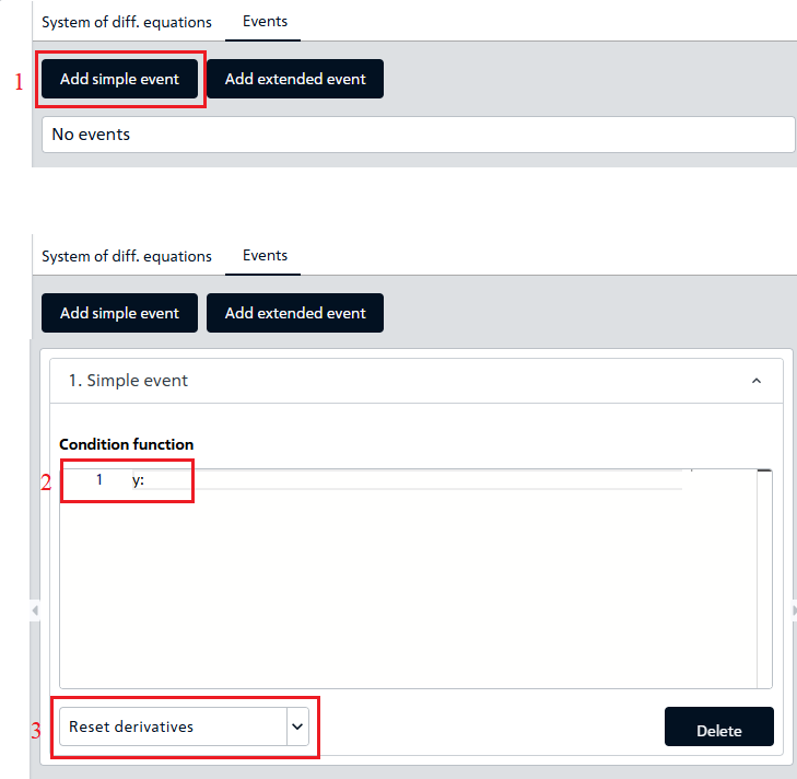
Fig. 12 Adding a new simple event

 In addition to the new event, the code for handling collisions was modified; changes were made to the Main block and After integration sections in Additional blocks:

Main block

if(L_OP_sensor<31) {
velocity' = -g*Math.sin(theta) -phi_VP*velocity*velocity*ro/2/m ;
l_OP'=2*phi_VP*velocity*velocity*ro/(Math.PI*mu*d_OP*d_OP*L_OP);
L_OP'= l_OP;
theta' = -g*Math.cos(theta)/velocity;
} else {
if(y>0) {
velocity' = -g*Math.sin(theta) - phi_OP*velocity*velocity*ro/2/m ;
theta' = -g*Math.cos(theta)/velocity;
if(gndHit==1){
velocity' = -g*Math.sin(theta);
}
} else {
double stiffness =1e4; 
double damping = 50;
velocity' = g  + stiffness*y - damping*velocity;
theta' = 0;
} 
l_OP'= 0;
L_OP'= 0;
}
x'=velocity*Math.cos(theta);
y'=velocity*Math.sin(theta);

• Lines 1-6. Block of code containing the equations for the first stage of landing, when the pilot chute is deployed. This block is executed until the main parachute fully deploys (L_OP_sensor<31);

• Lines 7-13. Block of code containing the equations for the second stage of landing when the main parachute opens. The calculation of the model in this block occurs when the main parachute is extended to its full length (L_{op} = 31). Subblock 10-13 contains the equation for the velocity after impact with the ground, when the drag force of the main parachute becomes zero;

• Lines 14-16. Block of code with the equations of the fourth stage, calculation of the model upon collision with the ground.

Additional blocks - After integration

velocity_sensor = velocity;
theta_sensor = theta;
x_sensor = x;
y_sensor = y;
L_OP_sensor = L_OP;
if(L_OP_sensor>31) {
L_OP = 31;
L_OP_sensor = L_OP;
}
u = (timer*velocity)/(n*D_OP);
if(u>1) { 
u = 1;
}
phi_OP = (c_OP*f_OP)*Math.pow(u, k);
if(y_sensor<0){
gndHit =1;
} 

• Lines 15-17. In the After Integration subsection, lines 15-17 are added, in which the variable gndHit signals a collision with the ground and is set to 1.

8.  Results of modeling a modified UAV landing model

 The graphs of the altitude and speed of the UAV before and after the collision with the ground have the form, Fig. 13:

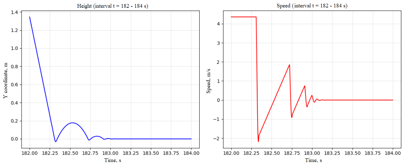
Fig. 13 Graphs of UAV landing altitude and speed

 The results of the calculation of the modified model demonstrate that the ODE block can work not only with continuous processes, but also with rigid systems, where the DE parameters change abruptly.

9.  Conclusions

 Within the framework of this manual, a mathematical model of parachute landing of an unmanned aerial vehicle of the aircraft configuration was successfully developed, implemented and verified on the REPEAT VISION platform using the ODE block.

1. Achieved results and model verification

The conducted study demonstrates the high efficiency and accuracy of using the ODE block for solving complex dynamic problems. The calculation results obtained on the REPEAT VISION platform correspond with high accuracy to the data given in the monographs (V.S. Moiseev [1], [2]), and serve as convincing evidence of the correctness of the model.

2. Functionality and reliability of the unit ODE

In the course of the work, the ability of the ODE block of the REPEAT VISION platform to stably solve ODE systems with intermittent dynamics was confirmed.

3. Practical significance and scope of application

The developed model is a ready-made tool for design calculations, allowing the trajectory and landing point of a UAV to be determined with high reliability.

10.  References

---

[1] (1,2,3,4,5,6)

Moiseev V.S. Flight dynamics and control of unmanned aerial vehicles: monograph. – Kazan: Editorial and publishing center “School”, 2017. 416 p.

[2] (1,2,3,4,5)

Moiseev V.S. Applied Theory of Unmanned Aerial Vehicle Control: Monograph. Kazan: Republican Center for Monitoring the Quality of Education (RC MKO), 2013. 768 p.

[3]

Reference REPEAT VISION platform: block ODE.