Determining the required water flow rate in a pipeline system#

Design of pipeline systems and their commissioning (commissioning) require both modeling and solving optimization problems.

Optimization problems can be solved to determine the parameters of a model for compliance with the TS of the designed pipeline system. This tutorial examines the problem of finding the area of the orifice plate to ensure the required water flow in a pipeline system.

Important

If you are not familiar with the category of inverse problems solved using the optimizer, it is recommended that you complete the basic tutorial before completing this tutorial.

During this tutorial you will learn:

With an example project for finding the required flow rate in a pipeline system, included in the set of DEMO projects for the REPEAT VISION platform;
With preliminary requirements for models of products and systems intended for solving optimization and research problems;
With the possibility of using a generalized approach to finding the root of the target function, which can be found in more detail in the relevant tutorial;
With the peculiarities of forming the boundaries of the set of admissible values of the parameters of the objective function.
With the capabilities of the optimization platform REPEAT VISION to solve the problem of finding the required flow rate in a pipeline system.

1. Project review to determine required flow rate in piping system#

To complete this tutorial, add the [DEMO] Finding required flow rate in pipeline system project from the Demo Projects folder of the REPEAT VISION platform to your project set.

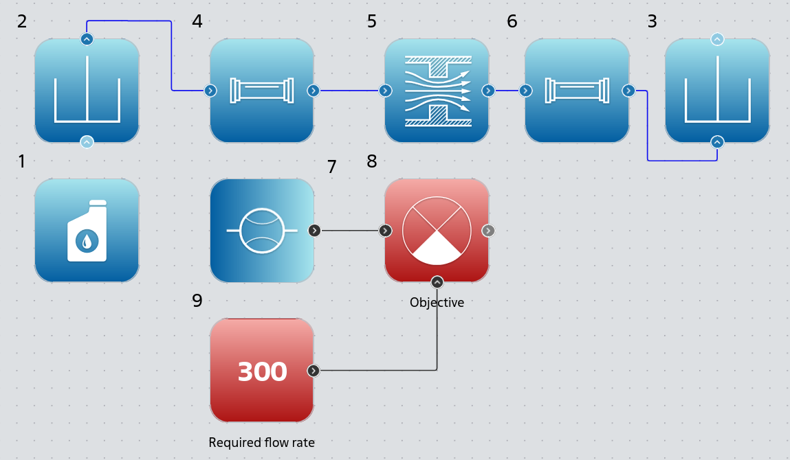
../../../_images/repeat_vision_project_find_flowrate.en.png — Project for determining the required flow rate in a pipeline system#

The project is designed to demonstrate a solution to a typical problem in the energy industry: ensuring the required water flow in a pipeline system by changing the hydraulic resistance at the throttle orifice (nozzle). This problem belongs to the category of inverse problems, solved using the optimization.

The project includes blocks of two libraries:

Isothermal hydraulics for calculating the mass flow rate of water in a pipeline system;
Automation for calculating the values of the objective function, intended to solve the optimization problem.

The example [DEMO] Finding required flow rate in pipeline system implements a stationary hydraulic model, for which the following project settings are used:

Simulation time [s]	Integration step [ms]	Sampling step [ms]
0.1	50	50

1.1. Hydraulic part of the model#

The hydraulic part of the project simulates the movement of fluid in a pipeline system consisting of two straight sections of pipeline and a throttle orifice (nozzle). The nipple creates hydraulic resistance to ensure the required water flow.

Block №1 Isothermal liquid properties (IH) is needed to set up the properties of water moving in the pipeline system. The block settings are set to default, except for the properties listed in the table below.

Property	Value
Related block	[2] Reservoir (IH)
Parameter	Output

Block №2 and block №3 Reservoir (IH) are necessary to determine constant values of boundary conditions for pressure at the inlet and outlet of the pipeline system. Blocks have property settings according to the table below.

Block	Gauge pressure, Pa
№2	100000.0
№3	0.0

Block №4 and block №6 Pipe (IH) are intended for calculating pressure losses during liquid flow in a pipeline system on straight sections of pipelines. Block №4 and block №6 use the same property values, listed in the table below.

Property	Value
Pipe length, m	10
Pipe diameter, m	0.2

The remaining settings of block №4 and block №6 are set to default.

Block №5 Orifice (IH) is designed to regulate the flow of liquid by changing the hydraulic resistance on the throttle orifice (fitting). The Port area, m² block property has a calculated expression 0.25*pi*0.2^2, corresponding to the area of a circular pipe opening with a diameter of 0.2 \([m]\) (see above the settings of block №4 and block №6). The block property Opening area, m² has a value of 0.001 to ensure water flow is greater than zero. The remaining block settings are set by default. The ‘Orifice area, m²’ property will be used by the optimization to modify the hydraulic resistance in order to find the required flow rate in the pipeline system.

1.2. Model objective function#

This part of the project is intended for the final calculation of the objective function optimization problem, the statement of which is given in the section below.

The required water flow rate of 300 \([kg/s]\), which must be ensured in the pipeline system in accordance with the problem statement, has been entered into the Constant value property of block №9 Constant.

Block №8 Signal difference (Controller error) is used by the optimizer as objective function. The block subtracts the calculated value of the water mass flow rate measured by block №7 from the required water flow rate specified in block №9.

1.3. Launching the project for calculation#

At the end of the project review, it is necessary to run the simulation to subsequently become familiar with the calculation results for the given hydraulic model settings.

As a result of the simulation, the mass flow rate of water in the pipeline system is 9.229802 \([kg/s]\).

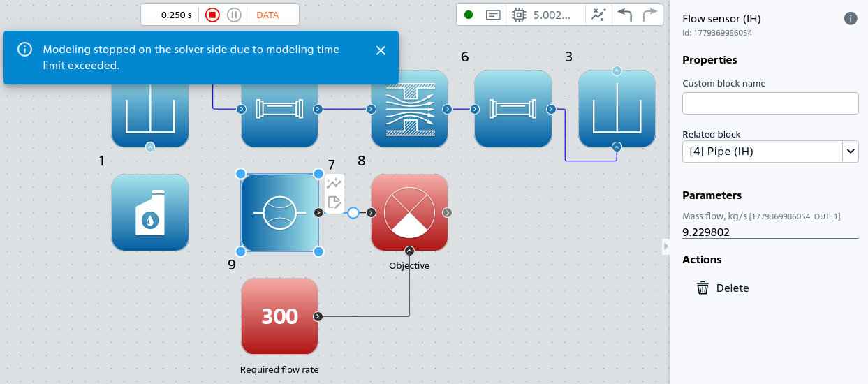
../../../_images/default_project_settings_results.en.png — Calculated value of water flow in the pipeline system with the initial model settings#

The water mass flow rate of 9.229802 \([kg/s]\) differs from the required flow rate by 290.7702 \([kg/s]\) (block №8 Signal difference (Controller error)). The model requires adjusting the hydraulic resistance on the throttle orifice (fitting) by changing the area of the hole block №5 Orifice (IH).

Tip

The empirical method of adjusting hydraulic resistance can take a long time to operate.

In order to reduce the labor costs of searching for the area of the nozzle opening and to increase the accuracy of ensuring the required flow rate in the pipeline system, it is necessary to use the optimization.

2. Statement of the optimization problem#

Before describing the formulation of the optimization problem, it should be noted that hydraulic modeling of a pipeline system is a direct problem (1) calculation of the mass flow rate of liquid \(m [kg/s]\) given the presence in the system model \(g\) of all necessary initial data \(x\): the boundary conditions for pressures are known, the properties of the liquid are known, the layout of the pipeline system is known, the design parameters are selected in advance, as well as the materials of the pipes and fittings.

(1)#\[m = g(x)\]

The problem under consideration of determining the required flow rate in a pipeline system is an inverse problem. The Inverse problem consists of determining the unknown value of the area of the orifice \(x [m^2]\) block №5 Orifice (IH) in the existing model of the pipeline system subject to the condition of fulfilling the equality (2) at a pre-known mass flow rate \(\text{const} [kg/s]\) equal to \(300 [kg/s]\) and fixed in block №9 [Constant]. The mass flow rate value may be a requirement of the TS.

(2)#\[g(x) = \text{const}\]

The Inverse problem is transformed into the problem of finding the root of \(x\) using the objective function \(f(x)\) (3).

(3)#\[\begin{split}\left\{ \begin{aligned} & f(x) = g(x) - \text{const} = 0 \\ & x \in \chi \end{aligned} \right.\end{split}\]

The rootfindhydro problem {eq} uses the following notation:

\(f\) is the objective function for which the root \(x\) must be found when \(f(x) = 0\);
\(g\) - pipeline system model for calculating the mass flow rate of water;
\(\text{const}\) - required value of mass flow rate \([kg/s]\);
\(x\) - area of the throttle orifice (fitting);
\(\chi\) is the set of permissible values of the nozzle opening area.

2.1. A set of acceptable values for the area of the nozzle opening#

The unknown area of the nozzle opening \(x [m^2]\) must belong to the set of admissible values \(\chi\). The set \(\chi\) must be limited taking into account the purpose of the nozzle, ensuring the required water flow rate:

The minimum value of the orifice area is 0.0001 \([m^2]\), at which the calculated value of the mass flow rate will be greater than zero, providing the optimizer with the minimum calculated value of the mass flow rate, \(m = g(0.0001) = 0.906 [kg/s]\);
The maximum value of the nozzle opening area 0.03 \([m^2]\) should not exceed the opening area of the connected sections of the pipeline to ensure the convergence of the hydraulic calculation (physically justified maximum value of the nozzle opening area), providing the optimizer with the maximum calculated value of the mass flow rate, \(m = g(0.03) = 401.569 [kg/s]\);

Hint

It can be noted that for a continuous function \(g(x)\), according to the Bolzano-Cauchy theorem, there exists an intermediate value of the area of the nozzle opening \(x \in [0.0001; 0.03]\), at which the mass flow rate of water \(g(x) = 300 [kg/s]\), \(300 \in [0.906; 401.569]\).

3. Configuring the optimizer#

To configure the optimizer, click the Optimization icon on the bottom panel of the REPEAT VISION user interface. In the tab that opens, apply the settings to solve the root search problem.

3.1. Main settings#

In the Main settings section, you need to apply the following settings.

Optimization task type	Optimization budget	Handling of non-physical values (NaN)
Root finding	25	Raise exception

Hint

For simple, smooth, continuous objective functions similar to quadratic functions, a small budget (\(10 \leq budget \leq 100\)) is sufficient to solve the root finding problem.

3.2. Optimization algorithm#

In the Optimization algorithm section, you need to apply the following settings.

Optimization method	Absolute tolerance of the varied parameter
Brent’s method	1e-15

In the Optimization method setting, you must select Brent's method to search for the root using the Brent method, which guarantees the convergence of the solution to the problem for the objective function, computable within the specified boundaries.

The setting Absolute tolerance of the varied parameter must be assigned a value of 1e-15 to fix the convergence criterion for the solution of the optimization problem for the area of the nozzle opening \(x\).

Note

It should be noted that the small value of 1e-15, close to the precision of a double in Java, is suitable for Brent's method and smooth, continuous objective functions.

3.3. Parameter settings#

In the Objective function calculation block setting, located in the Optimized parameters section, you must select the Output port of block №8 Signal difference (Controller error), which performs the final operation of calculating the objective function \(f(x)\).

In the Variable properties setting, located in the Varied block property section, you must select the Orifice area, m² property of block №5 Orifice (IH). The block hole area will be used by the optimizer as a variable parameter \(x\) to find the root of the objective function \(f(x)\) (see equation (3)).

You also need to specify the boundaries within which the root search is performed, in accordance with the rationale given in the section above. Thus, in the Min value field, you must enter 0.0001, and in the Max value field, you must enter 0.03.

3.4. Launch optimization#

After completing the optimizer setup, you need to run optimization. To run optimization, click the Optimize button.

After successfully completing the root search, it is necessary to analyze the obtained solution.

4. Analysis of optimization results#

The optimization results are available in the corresponding section for performing analysis after successful completion of the root search.

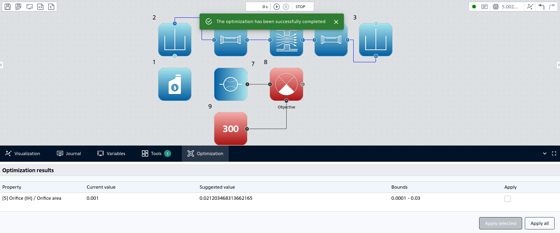
../../../_images/orifice_area_root_result.en.png — Results of searching for the area of the nozzle opening to ensure the required mass flow rate of water#

The optimizer determined the root of the objective function \(f(x)\) for the value of the nozzle opening area, \(x^{*} = 0.021203468313662165 [m^2]\), which belongs to the set of admissible values \(x \in [0.0001; 0.03]\).

Next, you need to click the Apply all button to transfer the root of the objective function \(x^{*}\) to the Orifice area, m² property of block №5 Orifice (IH). After clicking the button, a notification will appear indicating that the optimal properties have been successfully applied.

At the end of the analysis, it is necessary to run the calculation of the model with the optimal value of the nozzle opening area \(x^{*} = 0.021203468313662165 [m^2]\) and get the calculation result on the Output port of block №8 Signal difference (Controller error), which performs the final operation of calculating the target function \(f(x)\).

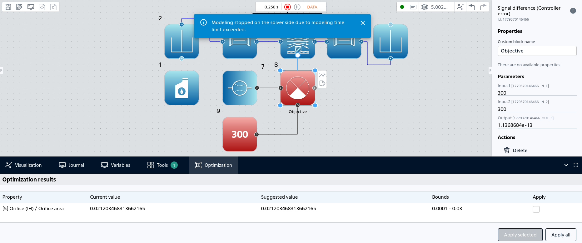
../../../_images/orifice_area_apply_result.en.png — The value of the objective function with the optimal area of the nozzle opening.#

The calculation result shows:

The calculated value of the mass flow rate of water \(g(x^{*}) = 300 [kg/s]\) at the port Input 1 block №8, obtained from the flow sensor - block №7;
The value of the objective function \(f(x^{*}) = 1.1368684e-13\) at the Output port of block №8.”

The calculated value of the mass flow rate corresponds to the required value of the mass flow rate of water \( 300 [kg/s]\) in the pipeline system with an optimal area of the nozzle opening \(x^{*} = 0.021203468313662165 [m^2]\).

5. Conclusions#

As a result of completing the practical guide to determining the required water flow rate in a pipeline system, you learned:

How to quickly and accurately solve a typical energy industry problem using the optimizer REPEAT VISION;
Features of the formation of physically justified boundaries of the set of admissible values of the parameters of the objective function.

To consolidate the experience gained, a generalized list of requirements for models designed to solve optimization problems is provided below.

5.1. General requirements for models designed to solve optimization problems#

When designing products and systems, optimization is always a task that follows the preparation of a system model and the analysis of the obtained calculation results. First, it is necessary to prepare a model of the product or system for conducting the main calculation.

The Model must be debugged. The model must be free of startup errors, and the calculation must complete successfully.

The model must contain blocks for calculating the objective function, and the model must also contain block properties that can be modified by the optimizer. Varying the block properties should result in changes in the objective function values.

During model debugging, it is recommended to conduct a series of computational experiments at the boundaries of the range of acceptable values for variable block properties. Calculations should complete successfully for both the minimum and maximum values of the block properties used to solve the optimization problem.