

Basic methods of parametric studies#
Before you practice the basic methods of parametric studies, one should consider the typical process, which is typical for all parametric studies.
Типовой процесс параметрических исследований модели системы на платформе REPEAT VISION/A typical process for parametric studies of a system model on the REPEAT VISION platform#
The model preparation I step will not be affected by this practical guide. One can familiarize oneself with this part of the process by completing the following two tutorials:
As part of the basic practical manual on parametric studies, you will learn:
Basic steps required to perform parametric studies on the REPEAT VISION platform;
Rules for choosing the parametric research method that is most suitable for your problem solution.
1. Review of sample model for parametric studies on the REPEAT VISION platform#
In order to learn how to perform parametric studies on the REPEAT VISION platform, add a simple example of isothermal hydraulics with the following name [DEMO] Local resistance pipeline from the Demo Projects folder to your project set.

Pipeline design with local resistance#
The example [DEMO] Local resistance pipeline allows investigating the change in fluid flow rate resulting from the calculation when the parameters given in the table change below.
Parameter |
Parameter type |
Global variable name |
Applies to block |
|---|---|---|---|
Tank pressure |
Boundary condition |
pressure |
block №1 |
Hole area in pipeline local resistance |
Structure parameter |
hole_area |
block №7 |
Diameter of pipeline sections |
Structure parameter |
pipe_diameter |
block №3 block №12 |
The result of the model calculation is transmitted to the block out_1 with the user name flowrate.
Proceed with the parametric study steps after reviewing the sample of pipeline model.
2. Parametric studies on the REPEAT VISION platform#
First open notebook and create a script in a new notebook to connect to the model via the REPEAT VISION platform.
Next, in the first cell, add the Python boot code repeat package, which is necessary for interacting with the REPEAT VISION platform and for performing parametric studies.
import piplite
await piplite.install("repeat")
In the next cell, import the Python packages needed to prepare the data for the studies, process the calculation results and then visualize the charts to analyze the research results.
import numpy as np
import pandas as pd
import matplotlib.pyplot as plt
In the next cell, import the Python repeat package with the parametric studies module.
1import repeat as rp
2import repeat.parametric_study as ps
Added in version 1.0.0: A module parametric_study is added to the new Python package version repeat to simplify parametric studies.
For more information about module parametric_study features, see Help.
Next, one needs to configure the connection to the REPEAT VISION platform and select a model to perform parametric studies.
user = rp.User(
  "enter a unique API key from REPEAT VISION user cabinet instead of this comment"
  )
app = rp.Application(user)
# enter a project ID from REPEAT VISION application instead of 12345
project = 12345
t_interval = rp.TimeInterval(start = 100, end = 200)
model = app.get_exploration_model(project, t_interval)
Let’s check the connection in the next cell, which can be deleted after debugging the program
print(model, model.existing_variables, sep = "\n")

# ExplorationModel(project = 12345, name = '[DEMO] Трубопровод с местным
# сопротивлением', time_interval = TimeInterval(start = 100, end = 200))
#
# hole_area            0.001
# pipe_diameter        0.200
# pressure         70000.000
# dtype: float64
The output of the print function shows that the name name of the instance of the ExplorationModel class of the selected model matches the model discussed in the figure above. Also, the list of existing_variables of global variables corresponds to the previously discussed model variable table.
Now everything is ready for choosing an algorithm for creating a parameter space.
2.1. Selection of parameter space creation algorithm#
One shall select an algorithm for creating a parameter space in order to perform parametric studies.
The choice of algorithm depends on the following criteria given in the table below.
Criterion |
Description |
|---|---|
The required sampling of calculation results |
A criterion for the real value of the pitch between the set of parameters \(\mathbf x_i\) and the set \(\mathbf x_{i+1}\). The choice of pitch depends on the nonlinearity of the \(\mathbf y = f(\mathbf x)\) function, which should be considered based on the results of a parametric study. The pitch is selected empirically. |
Duration of one calculation |
A criterion for the time spent on simulation with a limited total time for research. Long-term performance of each calculation directly affects the time spent on parametric studies. |
Dimension of the problem of parametric studies |
A criterion that comprises the number of variable parameters \(\mathbf n\) and the required number of calculations \(\mathbf m\). A large number of \(\mathbf n\) and \(\mathbf m\) results in a significant amount of time for parametric studies. |
In accordance with the criteria considered, the choice of the algorithm is reduced to one of the following options.
To be selected in the following cases:
A predetermined sampling of the calculation results with the assigned step for each of the model parameters is required;
Low duration of one calculation of the model relative to the specified time for performing studies;
Low dimension of the parametric study problem.
To be selected in the following cases:
High duration of one calculation of the model relative to the specified time for performing studies;
High dimension of the parametric study problem.
Algorithm selection for creating the parameter space for sample model#
One calculation of the sample model
[DEMO] Pipeline with local resistanceis performed in a short time (less than 1 second);The model contains only three global variables.
In order to perform parametric studies, in the first approximation, the algorithm for preparing a grid of parameter values is selected.
2.2. Preparation of data for studies#
Let’s set the next task of parametric studies. It is required to perform a parametric study when changing the parameters given in the table below.
Parameter |
Description |
Change boundaries |
Number of values |
|---|---|---|---|
|
Hole area in pipeline local resistance |
\([10^{-7}, 0.02] m^2\) |
6 |
|
Tank pressure |
\([10^4, 10^6] Pa\) |
5 |
In a parametric study it is not necessary to account for the parameter pipe_diameter, that is, its value will be constant, equal to \(0.2 m\).
Create a variable_values dictionary according to the requirements of the get_cartesian_product function for the algorithm for preparing a grid of parameter values in the following cell.
variable_values = dict(
    hole_area = np.linspace(1e-7, 0.02, num = 6),
    pressure = np.linspace(1e4, 1e6, num = 5),
    pipe_diameter = np.array([0.2]),
)
In the next cell, one needs to create a Cartesian product for a set of parameter values using the get_cartesian_product function of repeat.parametric_study module, which was imported as ps above. The ExplorationModel class is transferred to the function as the first argument and the variable_values dictionary containing sets of parameter values is transferred as the second argument.
input_data = ps.get_cartesian_product(model, variable_values)
m, n = input_data.shape
print("Размерность задачи:\n"
  f"Количество варьируемых параметров {n = };\n"
  f"Необходимое количество расчётов {m = }.\n"
)
input_data.head(2)
The following information appears at the cell output as a result of the parameter values grid preparation algorithm.
Dimension of the problem:
Number of variable parameters n = 3;
The required number of calculations m = 30.
hole_area |
pressure |
pipe_diameter |
|
|---|---|---|---|
0 |
1.000000e-07 |
10000.0 |
0.2 |
1 |
4.000080e-03 |
10000.0 |
0.2 |
As a result of the next cell performance, we obtain grid of values of hole_area and pressure parameters.
axis = input_data.plot.scatter(x = 'hole_area', y = 'pressure', c = 'tab:green')
axis.set_xlabel("hole_area $[m^2]$")
axis.set_ylabel("pressure $[Pa]$")
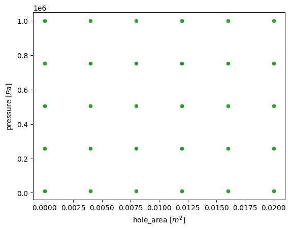
Grid of parameter values as a result of the function get_cartesian_product modulerepeat.parametric_study#
The chart shows the uniform covering with 30 values of pressure and hole_area parameters within the boundaries corresponding to the table above.
In the next cell, it is necessary to create the common table suitable to save the calculation results and the subsequent performance of the parametric study analysis.
design_cases = input_data.copy(deep = True)
design_cases["flowrate"] = pd.NA
design_cases.head(2)
hole_area |
pressure |
pipe_diameter |
flowrate |
|
|---|---|---|---|---|
0 |
1.000000e-07 |
10000.0 |
0.2 |
|
1 |
4.000080e-03 |
10000.0 |
0.2 |
|
The input_data table is copied to the new design_cases item and a new flowrate column is created to save the results of the model calculation.
Tip
It is recommended to always initialize the calculation results column with pd.NA or `np.nanfor values for subsequent parametric studies.
In case of successful calculation completion, a real value with the calculation result will be saved instead of pd.NA.
In case of problem occurrence, the user will have the information on the numbers of calculations (where the pd.NA values remained), in which it is necessary to perform additional debugging of your Python program or model.
2.3. Performing a model calculation cycle on the REPEAT VISION platform#
Then it is required to perform a cycle of model calculations on the REPEAT VISION platform. For this purpose let’s create the solve function and perform it in the next cell.
def solve(input_data, design_cases):
    for i, variables in input_data.iterrows():
        with model as md:
            md.run(variables)
            design_cases.loc[i, "flowrate"] = md.get_results("flowrate").iloc[-1]

solve(input_data, design_cases)
The solve function uses only one cycle, for which all 30 model calculations are performed.
Inside the cycle, using the with context manager, the model is started for calculation by the .run() method with the current variables set of global variable values.
Also, inside the context manager, the .get_results() method saves one actual value of the "flowrate" flow rate calculation result to the design_cases table at the end of the simulation time. This value is obtained by the .iloc[-1] method from the pandas.Series structure.
3. Analysis of the results of parametric studies on the grid of values#
It is required to create an auxiliary function of three-dimensional visualization based on the matplotlib package possibilities to display the results of calculations.
def plot_3d_scatter(table):
    fig = plt.figure()
    ax = fig.add_subplot(projection = "3d")
    ax.scatter(
        table["pressure"],
        table["hole_area"],
        table["flowrate"],
        marker='o'
      )
    ax.set_xlabel("pressure $[Pa]$")
    ax.set_ylabel("hole_area $[m^2]$")
    ax.set_zlabel("flowrate $[kg]$")
    plt.show()
In the next cell it is required to call this function to perform the analysis of the results on the grid of pressure and hole_area parameter values. The previously filled in design_cases table is transmitted to the plot_3d_scatter visualization function.
plot_3d_scatter(design_cases)
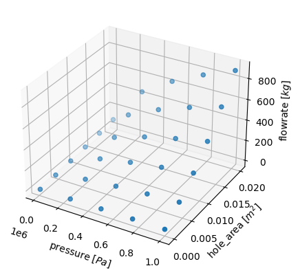
Results of calculating the mass flow rate flowrate on the grid of values parameters pressure and hole_area#
The three-dimensional picture of distribution of flowrate dependence on pressure and hole_area shows the increase of mass flow rate flowrateat increase of pressurepressureand increase of hole areahole_area`.
4. Code of the whole program for performance of parametric studies on the grid of parameter values#
Below there is a code of the above program for performance of parametric studies on the grid of parameter values for convenient use and copying.
import piplite
await piplite.install("repeat")

import numpy as np
import pandas as pd
import matplotlib.pyplot as plt
import repeat as rp
import repeat.parametric_study as ps


user = rp.User(
  "enter a unique API key from REPEAT VISION user cabinet instead of this comment"
  )
app = rp.Application(user)
# enter a project ID from REPEAT VISION application instead of 12345
project = 12345
t_interval = rp.TimeInterval(start = 100, end = 200)
model = app.get_exploration_model(project, t_interval)
print(model, model.existing_variables, sep = "\n")

variable_values = dict(
    hole_area = np.linspace(1e-7, 0.02, num = 6),
    pressure = np.linspace(1e4, 1e6, num = 5),
    pipe_diameter = np.array([0.2]),
)
input_data = ps.get_cartesian_product(model, variable_values)
m, n = input_data.shape
print("Размерность задачи:\n"
  f"Количество варьируемых параметров {n = };\n"
  f"Необходимое количество расчётов {m = }.\n"
)
input_data.head(2)

axis = input_data.plot.scatter(x = 'hole_area', y = 'pressure', c = 'tab:green')
axis.set_xlabel("hole_area $[m^2]$")
axis.set_ylabel("pressure $[Pa]$")

design_cases = input_data.copy(deep = True)
design_cases["flowrate"] = pd.NA
design_cases.head(2)

def solve(input_data, design_cases):
    for i, variables in input_data.iterrows():
        with model as md:
            md.run(variables)
            design_cases.loc[i, "flowrate"] = md.get_results("flowrate").iloc[-1]

solve(input_data, design_cases)

def plot_3d_scatter(table):
    fig = plt.figure()
    ax = fig.add_subplot(projection = "3d")
    ax.scatter(
        table["pressure"],
        table["hole_area"],
        table["flowrate"],
        marker='o'
      )
    ax.set_xlabel("pressure $[Pa]$")
    ax.set_ylabel("hole_area $[m^2]$")
    ax.set_zlabel("flowrate $[kg]$")
    plt.show()

plot_3d_scatter(design_cases)
5. Application of algorithm for preparation of sparse set of parameter values#
Let’s use the current model sample to obtain basic skills in using the algorithm for preparing a sparse set of parameter values.
In the next cell of the current parametric study program, let’s create a variable_bounds dictionary in accordance with the requirements of the get_latin_hypercube function for parameters with the boundaries of the values given in table above.
variable_bounds = dict(
    hole_area = [1e-7, 0.02],
    pressure = [1e4, 1e6],
    pipe_diameter = 0.2,
)
Note that the get_latin_hypercube function does not requires creating an initial set of values, as is required for the get_cartesian_product function, but only the lower and upper values of the parameter boundaries shall be specified.
The existing formulation of the parametric study problem does not require varying the pipe_diameter parameter, therefore, it is indicated simply by the real value 0.2 in the variable_bounds dictionary.
Next, one needs to create a sparse set of values of global variables using the Latin hypercube method using the get_latin_hypercube function.
1lhs_input_data = ps.get_latin_hypercube(
2  model,
3  variable_bounds,
4  seed = 7,
5  sample_size = 16,
6  strength = 1,
7  optimization = "random-cd"
8  )
9lhs_input_data.head(2)
hole_area |
pressure |
pipe_diameter |
|
|---|---|---|---|
0 |
0.006205 |
443808.090862 |
0.2 |
1 |
0.009417 |
564156.088257 |
0.2 |
The ExplorationModel class sample is transferred to the function as the first argument and the previously created variable_bounds dictionary as the second argument, which contains the lower and upper values of the parameter boundaries.
Also, the named parameter sample_size is transferred to the function with the value 16 of the number of necessary parametric studies, which will then need to be performed. The strength and optimization settings are needed to control the uniformity of the parameter value space filling in, and seed is needed in case of debugging or if it is necessary to ensure the repeatability of a random set of global variable values.
5.1. Comparison of the algorithm for preparing a sparse set with the algorithm for preparing a grid of parameter values#
In order to compare different algorithms for preparing parameter value sets, one needs to execute in the next cell the mapping code for the distribution of hole_area and pressure parameter values obtained earlier by the get_cartesian_product function and the get_latin_hypercube function.
axis = input_data.plot.scatter(x = 'hole_area', y = 'pressure', c = 'tab:green')
lhs_input_data.plot.scatter(x = 'hole_area', y = 'pressure', c = 'tab:orange', ax = axis)
axis.set_xlabel("hole_area $[m^2]$")
axis.set_ylabel("pressure $[Pa]$")
The following designations are taken in the chart below.
Labels |
Description |
|---|---|
Green Labels |
Grid of parameter values obtained by Cartesian product of the original sets using the |
Orange labels |
A sparse set of parameter values obtained using the `get_latin_hypercube function |
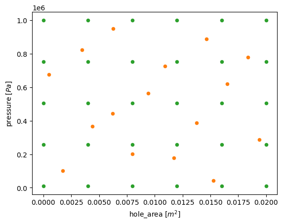
Graph of the distribution of parameter values as a result of the work of two algorithms: 1. Algorithm for preparing a sparse set of valuesparameters; 2. Algorithm for preparing a grid of parameter values#
The chart above shows that the set of values obtained by the get_latin_hypercube function in points sufficiently evenly fills the space of values for sample_size = 16 parameter sets.
Caution
As a drawback of the algorithm for preparing a sparse set using the Latin hypercube method, it should be noted that set of parameter values does not have values directly at the parameter boundaries, which may be important when assessing critical modes of system operation.
5.2. Performing a model calculation cycle on the REPEAT VISION platform#
In the next cell, let’s create a general table to save the calculation results and then perform the analysis of parametric studies (Description of the need for such an action was previously given in the section Preparation of data for studies).
lhs_design_cases = lhs_input_data.copy(deep = True)
lhs_design_cases["flowrate"] = pd.NA
Next, let’s perform a cycle of calculations of the model on the REPEAT VISION platform using the previously created solve function.
solve(lhs_input_data, lhs_design_cases)
5.3. Analysis of the results of parametric studies for the algorithm for preparing a sparse set of parameter values#
In the next cell, call the plot_3d_scatter function to visualize the calculation results obtained on a sparse set of parameter values.
plot_3d_scatter(lhs_design_cases)
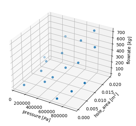
Results of calculating the mass flow rate flowrate on a sparse setvalues of the pressure and hole_area parameters”#
Despite the fairly good uniformity of the coverage of the space of parameter values, it is obvious that there are not enough results of the mass flow rate flowrate at the boundaries of the parameter values of pressure and hole_area parameters, as noted above in section Comparison of the algorithm for preparing a sparse set with the algorithm for preparing a grid of parameter values.
5.4. Code of the whole program for preparation of sparse set of parameter values#
For the convenience of review and copying, below there is a code of the above program for performing parametric studies on a sparse set of parameter values. The code for initializing interaction with the REPEAT VISION platform is given in the section Code of the whole program for performance of parametric studies on the grid of parameter values.
variable_bounds = dict(
    hole_area = [1e-7, 0.02],
    pressure = [1e4, 1e6],
    pipe_diameter = 0.2,
)
lhs_input_data = ps.get_latin_hypercube(
  model,
  variable_bounds,
  seed = 7,
  sample_size = 16,
  strength = 1,
  optimization = "random-cd"
  )
lhs_input_data.head(2)

axis = input_data.plot.scatter(x = 'hole_area', y = 'pressure', c = 'tab:green')
lhs_input_data.plot.scatter(x = 'hole_area', y = 'pressure', c = 'tab:orange', ax = axis)
axis.set_xlabel("hole_area $[m^2]$")
axis.set_ylabel("pressure $[Pa]$")

lhs_design_cases = lhs_input_data.copy(deep = True)
lhs_design_cases["flowrate"] = pd.NA
solve(lhs_input_data, lhs_design_cases)
plot_3d_scatter(lhs_design_cases)
6. Combining the procedure for preparing a sparse set of values with the procedure for preparing a grid of parameter values#
Let’s try to combine the two methods as follows. For boundary parameter values, let’s create 4 parameter sets on the grid: 2 sets for hole_area and 2 for pressure.
grid_input_data = ps.get_cartesian_product(
    model,
    variable_values = dict(
        hole_area = np.linspace(1e-7, 0.02, num = 2),
        pressure = np.linspace(1e4, 1e6, num = 2),
        pipe_diameter = np.array([0.2]),
    )
)
Next, using the algorithm for preparing a sparse set of values, create 16 sets of parameters, as in section above.
lhs_input_data = ps.get_latin_hypercube(
    model,
    variable_bounds = dict(
        hole_area = [1e-7, 0.02],
        pressure = [1e4, 1e6],
        pipe_diameter = 0.2,
        ),
    seed = 7,
    sample_size = 16,
    strength = 1,
    optimization = "random-cd"
  )
In the next step, let’s combine parameter sets into a common input data table for parametric studies.
input_data = pd.concat(
  [grid_input_data, lhs_input_data],
  ignore_index = True
  )
design_cases = input_data.copy(deep = True)
design_cases["flowrate"] = pd.NA
input_data.shape()
#
# (20, 3)
20 sets of values for parametric studies are formed above as a result of cell execution.
Now, having executed the cell below, let’s look at the resulting set of values for the hole_area and pressure parameters.
axis = grid_input_data.plot.scatter(x = 'hole_area', y = 'pressure', c = 'tab:green')
lhs_input_data.plot.scatter(x = 'hole_area', y = 'pressure', c = 'tab:orange', ax = axis)
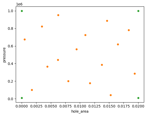
Distributions of values of the combined set of parameters#
The chart above shows that we got a sparse set of values in the availability of values at the boundaries of the space of parameter values.
Next, one needs to perform the calculation for subsequent analysis, which can be done using the three-dimensional picture of the distribution of the calculation results shown in Figure below.
solve(input_data, design_cases)
plot_3d_scatter(design_cases)
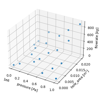
Results of calculating the mass flow rate flowrate on the combined set values of the pressure and hole_area parameters”#
As a result, on sufficiently evenly distributed space of parameter values, the results of calculating the mass flow rate flowrate were obtained on 20 sets of values (versus 30 sets of values obtained using the grid preparation algorithm) with a savings of 30% in the dimension of the research problem that affects the duration of parametric studies.
6.1. Code of the entire program for combining the procedure for preparing a sparse set of values with the procedure for preparing a grid of parameter values#
For the convenience of review and copying, below there is a the code of the above program for combining the procedure for preparing a sparse set of values with the procedure for preparing a grid of parameter values. The code for initializing interaction with the REPEAT VISION platform is given in the section Code of the whole program for performance of parametric studies on the grid of parameter values.
grid_input_data = ps.get_cartesian_product(
    model,
    variable_values = dict(
        hole_area = np.linspace(1e-7, 0.02, num = 2),
        pressure = np.linspace(1e4, 1e6, num = 2),
        pipe_diameter = np.array([0.2]),
    )
)
lhs_input_data = ps.get_latin_hypercube(
    model,
    variable_bounds = dict(
        hole_area = [1e-7, 0.02],
        pressure = [1e4, 1e6],
        pipe_diameter = 0.2,
        ),
    seed = 7,
    sample_size = 16,
    strength = 1,
    optimization = "random-cd"
  )
input_data = pd.concat(
  [grid_input_data, lhs_input_data],
  ignore_index = True
  )
design_cases = input_data.copy(deep = True)
design_cases["flowrate"] = pd.NA
input_data.shape()

axis = grid_input_data.plot.scatter(x = 'hole_area', y = 'pressure', c = 'tab:green')
lhs_input_data.plot.scatter(x = 'hole_area', y = 'pressure', c = 'tab:orange', ax = axis)

solve(input_data, design_cases)
plot_3d_scatter(design_cases)
7. Conclusions#
In the results of the step-by-step implementation of this practical guide, we obtained:
Recommendations for choosing a method for parametric studies;
Understanding of the advantages and disadvantages of the considered algorithms for preparing sets of parameter values;
Recommendations on application of algorithms for preparation of parameter value sets;
Understanding of the basic steps required to perform parametric studies on the REPEAT VISION platform.