Approximating the solution of an oscillation differential equation using PINN#

This tutorial provides instructions for creating a PINN — a Physics-informed neural network — to simulate the oscillation dynamics of a system, training it using physical laws, and exporting it to the ONNX format. The integration of the resulting model into the REPEAT VISION platform for calculations is demonstrated.

The tutorial consists of the following steps:

General problem description
Mathematical problem formulation
Building the PINN model in PyTorch
Exporting the model to ONNX format
Creating a project on the REPEAT VISION platform
Conclusions

1. Problem description#

The problem models the oscillation dynamics of a mechanical system representing a point mass attached to an elastic spring with a damper. The schematic of the mechanical system is shown in the figure below.

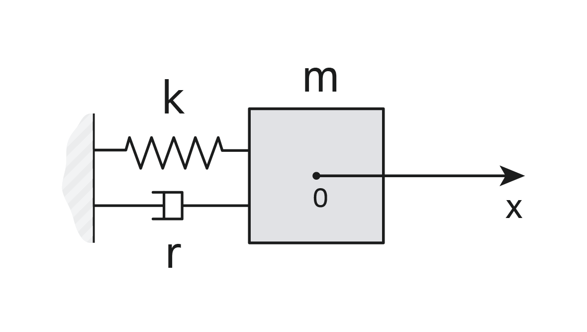
../../../../../_images/spring-mass-schema-a9c71caa.png — The schematic of the mechanical system#

The table below presents the notations used in the scheme.

Notation	Description	Units of measurement
\(\mathbf m\)	Mass of the object	\([kg]\)
\(\mathbf k\)	Spring stiffness coefficient	\([N/m]\)
\(\mathbf r\)	Damper resistance coefficient	\([N·s/m]\)
\(\mathbf x\)	Coordinate axis along which the object moves	\([m]\)

The object is displaced from equilibrium and released without initial velocity, allowing observation of damped oscillations caused by elastic and damping forces. This system models a typical oscillatory process without accounting for gravity.

System parameters

The object has a mass \( m = 1.0 \) kg.
The spring has a coefficient of elasticity \( k = 50.0 \) N/m, it determines the force that returns the object to the equilibrium position.
The damper has a resistance coefficient of \( r = 2.0 \) N·s/m, which results in damping of oscillations.

Initial conditions

The object is moved from the equilibrium position by \( x_0 = 2.0 \) m.
When released, the object has no initial velocity (\( v_0 = 0.0 \) m/s).

Simulation time interval

The simulation takes place over \( 10 \) seconds, which allows us to trace the damping of oscillations

2. Mathematical problem formulation#

The solved equation of the system’s oscillation dynamics is a homogeneous linear second-order differential equation with constant coefficients. Its analytical solution is derived for subsequent comparison.

The original differential equation is described by the formula (1):

(1)#\[m \, \ddot{x}(t) + r \, \dot{x}(t) + k \, x(t) = 0,\]

where:

\( m \), \( r \), \( k \) — parameters described in the table above,
\( x(t) \) — system displacement at time \( t \) [s],
\( \dot{x}(t) \) — first derivative of \( x \) with respect to time [m/s],
\( \ddot{x}(t) \) — second derivative of \( x \) with respect to time [m/s\(^2\)].

For convenience in preparing the Machine learning model, the equation (1) is divided by \( m \), yielding equation (2).

(2)#\[\ddot{x}(t) + \frac{r}{m} \, \dot{x}(t) + \frac{k}{m} \, x(t) = 0.\]

Introducing the notations:

Natural frequency: \(\omega_0 = \sqrt{\frac{k}{m}}\),
Damping coefficient: \(\gamma = \frac{r}{2m}\).

The equation (2) then takes the form:

\[ \ddot{x}(t) + 2\gamma \, \dot{x}(t) + \omega_0^2 \, x(t) = 0. \]

Assuming the solution has the form \( x(t) = e^{\lambda t} \). Substituting this into the equation yields the characteristic equation:

\[ \lambda^2 + 2\gamma \, \lambda + \omega_0^2 = 0. \]

The roots of the quadratic equation are:

\[ \lambda_{1,2} = -\gamma \pm \sqrt{\gamma^2 - \omega_0^2}. \]

Depending on the relationship between \( \gamma^2 \) and \( \omega_0^2 \) , three cases are distinguished: aperiodic damping, weak damping, and the critical case.

To determine the mode, we will substitute specific system parameters and consider the comparison \( \gamma^2 \) and \( \omega_0^2 \):

\[ \gamma^2 = (\frac{r}{2m})^2 = 1.0^2 = 1.0,\quad \omega_0^2 = \frac{k}{m} = 50.0. \]

Since

\[ \gamma^2 < \omega_0^2, \]

then in this case the solution of the equation is damped oscillations - a case of weak damping.

The frequency of damped oscillations, \( \omega_1 \) is defined by the formula (3).

(3)#\[\omega_1 = \sqrt{\omega_0^2 - \gamma^2}.\]

The general solution has the form of equation (4).

(4)#\[x(t) = e^{-\gamma t} \Big( A \cos(\omega_1 t) + B \sin(\omega_1 t) \Big).\]

The constants \( A \) and \( B \) are determined from the initial conditions:

\[ x(0) = x_0, \quad \dot{x}(0) = v_0. \]

Substituting \( t = 0 \) into the general solution:

\[ x(0) = A = x_0. \]

For the derivative:

\[ \dot{x}(t) = -\gamma e^{-\gamma t} (A \cos(\omega_1 t) + B \sin(\omega_1 t)) + e^{-\gamma t} \Big( -A \omega_1 \sin(\omega_1 t) + B \omega_1 \cos(\omega_1 t) \Big). \]

At \( t=0 \):

\[ \dot{x}(0) = -\gamma A + B \omega_1 = v_0. \]

From here we find:

\[ B = \frac{v_0 + \gamma x_0}{\omega_1}. \]

Thus, the final solution is given by equation (5).

(5)#\[x(t) = e^{-\gamma t} \left( x_0 \cos(\omega_1 t) + \frac{v_0 + \gamma x_0}{\omega_1} \sin(\omega_1 t) \right).\]

The graph of the point mass displacement for damped oscillations, according to the analytical solution (5), is shown in the figure below.

(png, hires.png)

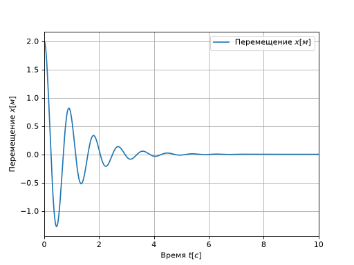
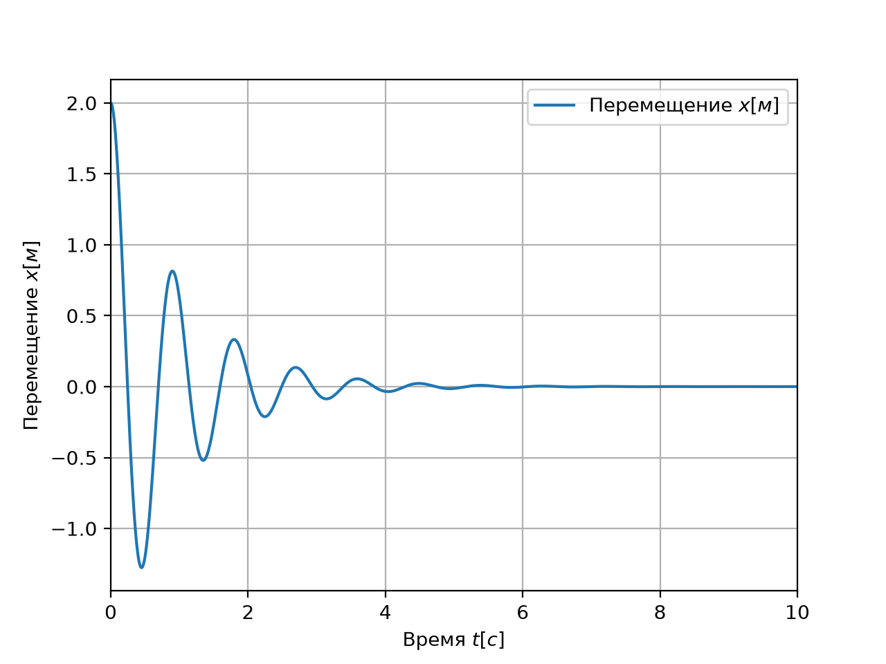
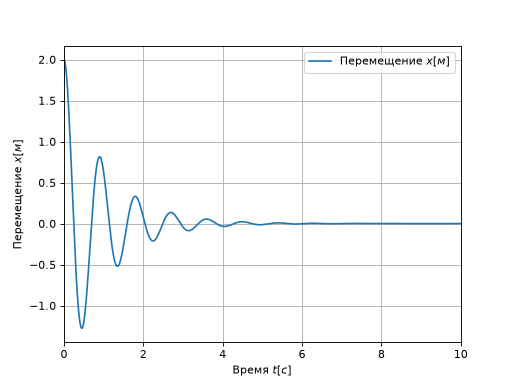
../../../../../_images/plots_plot_analytical_solution.png — Displacement of a point mass during damped oscillations#

3. Building the PINN Model in Python#

To solve the problem of modeling the oscillation dynamics using machine learning, a neural network with a modified loss function will be used. The modified loss function calculates the residual between the model’s predictions and equation (2). Neural networks incorporating such modified loss functions are called Physics-Informed Neural Networks (PINN).

Creating Physics-Informed Neural Networks does not require tabular input data. Only the mathematical description of the problem is needed.

Note

In the loss function of other neural networks, the difference between predicted values and reference values (provided as tabular data) is typically calculated.

For more details on Physics-Informed neural networks, refer to the corresponding practical guide.

The PINN model will be implemented in Python using the PyTorch framework. Basic knowledge of Python and PyTorch is required.

3.1. Preparing for work#

Note

You can download the Jupyter notebook file to quickly execute this tutorial on your computer.

Alternatively, you can download the PINN model file and immediately use it in a REPEAT VISION project with the Approximation Model block.

Before you start working, you need to install the necessary libraries. To do this, it is recommended to create a virtual environment. To do this, create a folder, for example, named repeat. In the working folder repeat, a virtual environment is created with the name nn_venv.

mkdir repeat
cd repeat
python -m venv nn_venv.

After creating the working folder and virtual environment, the virtual environment is activated. For Linux-based operating systems, the bash command is executed, and for Windows, the PowerShell command is executed.

bash

source nn_venv/bin/activate

PowerShell

nn_venv\Scripts\activate

Now install the packages: torch, onnx, pandas. This command will also install the necessary dependencies.

python -m pip install torch pandas onnx

Important

To install a PyTorch version supporting GPU and compatible with your CUDA version, visit the official website: https://pytorch.org/get-started/locally/.

A brief overview of the required packages is provided in the table below.

Package	Description
torch	The Pytorch package is required for creating the PINN model.
onnx	The ONNX package is required for exporting the neural network model to a neutral format for use on the REPEAT VISION platform.
pandas	The pandas package is required for analyzing simulation results.
json	Package for writing auxiliary data about the neural network model.

3.2. Creating the PINN Model Class#

First, import the necessary libraries for creating neural networks and subsequent export to ONNX format.

Importing required libraries#

import torch
import torch.nn as nn
import pandas as pd
import onnx
import json

Next, define the neural network architecture. The PINN class is a fully connected network consisting of several linear layers with the hyperbolic tangent (Tanh) activation function. The model takes time as input and outputs the predicted system displacement coordinate.

PINN class#

class PINN(nn.Module):
    """
    Физически-информированная нейронная сеть (PINN) для моделирования динамики колебаний.

    Аргументы:
        layers: list
            Список размеров слоёв нейронной сети.
    Методы:
        forward: torch.Tensor -> torch.Tensor
            Прямой проход через сеть, возвращающий предсказанные значения для входного времени.
    """
    def __init__(self, layers: list):
        super().__init__()
        self.layers = nn.ModuleList()
        for i in range(len(layers) - 1):
            self.layers.append(nn.Linear(layers[i], layers[i + 1]))
        self.activation = nn.Tanh()

    def forward(self, t: torch.Tensor) -> torch.Tensor:
        inputs = t
        for layer in self.layers[:-1]:
            inputs = self.activation(layer(inputs))
        x = self.layers[-1](inputs)
        return x

Line 1. Declaration of the PINN class, inheriting from the base class nn.Module of the PyTorch library. This provides access to built-in mechanisms for constructing and training neural networks.
Line 12. Declaration of the initialization method, which accepts a layers argument of type list, defining the number of neurons for each layer.
Line 13. Initialization of the base class nn.Module to configure internal PyTorch mechanisms, necessary for working with neural networks.
Line 14. Initialization of the ModuleList object to store the layers of the neural network. Using ModuleList automatically registers the parameters of all added layers.
Lines 15-16. Loop through the layers list (excluding the last element). For each pair of consecutive elements, a linear layer (nn.Linear) is created, where layers[i] is the input size and layers[i+1] is the output size. Each layer is added to ModuleList.
Line 17. Initialization of the Tanh activation function for hidden layers.
Line 19. Creation of the forward method, which defines the data flow through the network. It takes a tensor t (time data) and returns the model’s prediction (displacement).
Line 20. Creation of the inputs variable for input data, which is sequentially transformed by each layer.
Lines 21-22. Loop to pass data through all layers except the last one, as a nonlinear activation function needs to be applied to them. In the loop, each hidden layer processes the input tensor, and the activation function is applied to the result. The updated tensor value is stored in the inputs variable for passing to the next layer.
Line 23. Processing of data by the output layer without activation.

Next, define the model parameters according to the problem formulation.

Model parameters#

m = 1.0      # Масса системы
k = 50.0     # Коэффициент упругости
r = 2.0      # Коэффициент демпфирования
x_0 = 2.0    # Начальное смещение
v_0 = 0.0    # Начальная скорость
T = 10.0     # Общее время моделирования

3.3. Defining the loss function#

The loss function includes three components, described in the table below.

№	Component	Description
1	Initial displacement loss	Compares the predicted value at time 0 with \( x_0 \).
2	Initial velocity loss	Compares the derivative of the predicted value at time 0 with \(v_0 \).
3	Equation of motion loss	Residual calculated from the differential equation \( \ddot{x}(t) + \frac{r}{m} \dot{x}(t) + \frac{k}{m} x = 0 \).

The Python code for calculating the loss function is provided below.

Loss function#

def loss_function(model: PINN,
                  t_f: torch.Tensor,
                  t_i: torch.Tensor) -> torch.Tensor:
    """
    Вычисляет функцию потерь для модели PINN по уравнению колебаний.

    Параметры:
        model: PINN
            Обучаемая модель PINN.
        t_f: torch.Tensor
            Точки времени для вычисления остатка уравнения движения.
        t_i: torch.Tensor
            Точка времени для начальных условий (обычно t = 0).

    Возвращает:
        tuple: (loss, (loss_x0, loss_v0, loss_f))
            Общая функция потерь и отдельные составляющие: потери для начального смещения, начальной скорости и уравнения движения.
    """
    x_f = model(t_f)
    x_i = model(t_i)

    # Вычисление первой и второй производной для точек t_f
    x_f_t = torch.autograd.grad(x_f, t_f,
                                grad_outputs=torch.ones_like(x_f),
                                create_graph=True)[0]
    x_f_tt = torch.autograd.grad(x_f_t, t_f,
                                 grad_outputs=torch.ones_like(x_f_t),
                                 create_graph=True)[0]

    # Производная в точке t_i для начальных условий
    x_i_t = torch.autograd.grad(x_i, t_i,
                                grad_outputs=torch.ones_like(x_i),
                                create_graph=True)[0]

    # Глобальные параметры системы: m, r, k, x_0, v_0
    f = x_f_tt + (r/m) * x_f_t + (k/m) * x_f

    loss_f = torch.mean(torch.squeeze(f)**2)
    loss_x0 = torch.mean((torch.squeeze(x_i) - x_0)**2)
    loss_v0 = torch.mean((torch.squeeze(x_i_t) - v_0)**2)

    # Коэффициенты для балансировки вклада разных потерь
    coeff0, coeff1, coeff2 = 1, 1e-1, 1e-3
    loss = coeff0 * loss_x0 + coeff1 * loss_v0 + coeff2 * loss_f

    return loss, (loss_x0.item(), loss_v0.item(), loss_f.item())

Lines 1-3. Declaration of the loss_function, which takes the model, time points for residual calculation, and a single time point for initial condition validation as arguments. Returns a tuple: total loss value and individual loss components (initial displacement error, initial velocity error, and residual equation error).
Lines 19-20. Calculation of the model’s output (displacement) for time points t_f via the forward method (it is made available by inheriting the PINN class from nn.Module). Similarly, the output for t_i is calculated.
Lines 23-33. Calculation of the first and second derivatives for t_f using torch.autograd.grad. The grad_outputs=torch.ones_like(x_f) parameter indicates the derivative is calculated for each element of x_f. create_graph=True enables further differentiation, which is necessary to calculate the second derivative. The reference to [0] is used to extract the gradient tensor itself from the returned tuple.
Lines 31-33. The second derivative of the model output with respect to time is calculated in a similar way for the points t_f, for this purpose the already calculated first derivative x_f_t is used.
Lines 36. Calculation of the oscillation equation residual, where all derivatives and problem parameters are substituted into the equation. If the model’s predictions satisfy the physical equation, \( f \) should tend to zero.
Lines 38-40. Calculation of the mean squared error of the equation residual and initial conditions, providing a measure of the model’s inconsistency with the problem. Using torch.squeeze(f) removes extra dimensions.
Lines 43-44. Introduction of weighting coefficients coeff0, coeff1, coeff2 into the loss function allows balancing the contribution of each component to the total loss. These coefficients are determined empirically.

3.4. Model configuration and training#

To train the model, create time points \(t[s]\) on the simulation time interval. Such points are called collocation points.

Parameter	Description
`t_f`	Points at which the equation of motion residual is calculated (linearly distributed from \( 0 \) to \( T = 10.0\)).
`t_i`	Point for checking initial conditions (\( t = 0 \)).

Important

Since many models lack extrapolation properties, the model must be trained on all values from the same intervals from which data will later be fed into it during modeling in REPEAT VISION. In other words, there should be no situation where the model in REPEAT VISION receives values outside the boundaries of the training dataset.

To speed up subsequent computations, define the available device (GPU, if available, or CPU). Declare the model class with the specified architecture and optimizer, and define the points for the equation and initial condition.

Declaring variables and classes#

device = torch.device('cuda' if torch.cuda.is_available() else 'cpu')

# Определение архитектуры сети: входной слой, 4 скрытых слоя по 32 нейрона и выходной слой
layers = [1, 32, 32, 32, 32, 1]
model = PINN(layers).to(device)

# Оптимизатор Adam с указанной скоростью обучения
optimizer = torch.optim.Adam(model.parameters(), lr=4e-3)

# Генерация точек времени для обучения
N_f = 1000  # Количество точек коллокации для уравнения
t_f = torch.linspace(0, T, N_f, device=device).view(-1, 1).requires_grad_(True)

t_i = torch.tensor(0., device=device).view(-1, 1).requires_grad_(True)

Line 1. Definition of the computing device. If a CUDA-supported GPU is available, 'cuda' is used; otherwise, 'cpu' is used. This speeds up model training on GPUs if available.
Lines 4-5. Creation of the layers list, specifying the sizes of the network layers. The first element (1) corresponds to the input layer dimension, the next four values (32, 32, 32, 32) are the sizes of the hidden layers, and the last element (1) is the size of the output layer. Then, an instance of the PINN class is created using the previously defined layers list. The model is then moved to the device (GPU or CPU) for subsequent computations.
Line 8. Initialization of the Adam optimizer. The model parameters model.parameters() and the learning rate are passed as arguments.
Line 11. Definition of the variable N_f, specifying the number of collocation points for calculating the equation of motion residual.
Line 12. Generation of a linearly distributed tensor t_f of N_f points from 0 to \( T = 10.0\) using the specified device device. The view(-1, 1) method reshapes the tensor into a column, and requires_grad_(True) enables gradient computation, which is necessary for automatic differentiation when checking the equation.
Line 14. Creation of the t_i tensor from a single element \( t = 0 \) for checking initial conditions. The tensor is also moved to the device, reshaped into a column, and gradient computation is enabled.

Proceed to train the model. The main training loop runs for a specified number of epochs (e.g., 20000 epochs). In each cycle:

Gradients are zeroed.
The loss function is computed.
Backpropagation is performed.
Model parameters are updated.
The loss value is periodically printed to monitor the training process.

Training loop#

num_epochs = 20000

for epoch in range(num_epochs + 1):
    optimizer.zero_grad()
    loss, losses = loss_function(model, t_f, t_i)
    loss.backward()
    optimizer.step()

    if epoch % 1000 == 0:
        print(f'Epoch {epoch},',
              f'Loss_x0 = {round(losses[0], 4)},',
              f'Loss_v0 = {round(losses[1], 4)},',
              f'Loss_f = {round(losses[2], 4)}')

print("Обучение модели завершено.")

# Epoch 0, Loss_x0 = 4.2735, Loss_v0 = 0.0023, Loss_f = 19.1911
# Epoch 1000, Loss_x0 = 0.0001, Loss_v0 = 0.0341, Loss_f = 12.5342
# ...
# Epoch 10000, Loss_x0 = 0.0, Loss_v0 = 0.0, Loss_f = 0.2306
# ...
# Epoch 20000, Loss_x0 = 0.0, Loss_v0 = 0.0002, Loss_f = 0.0636
# Обучение модели завершено.

Line 1. Definition of the variable num_epochs, specifying the total number of training epochs.
Lines 3-13. The main model training loop. In each epoch:
- Optimizer gradients are zeroed.
- The loss function is computed using the previously defined loss_function.
- Backpropagation is performed to compute gradients for the model parameters.
- Model parameters are updated using the Adam optimizer.
- A condition checks if the current epoch is a multiple of 1000. This is used to periodically print training progress information.

Next, plot the approximated displacements from the PINN model.

Plotting Displacements from the PINN Model#

displacement = model(t_f)
approx_data = pd.DataFrame(dict(
    time = t_f.detach().numpy().flatten(),
    displacement = displacement.detach().numpy().flatten(),
))
axis = approx_data.plot(
    y = "displacement", 
    x = "time", 
    color = "tab:red", 
    label = "Перемещение $x [м]$"
    )
axis.set_ylabel("Перемещение $x [м]$")
axis.set_xlabel("Время $t [с]$")
axis.set_xlim(0, 10)
axis.grid(True)

Line 1. Calculation of approximated displacement values from the PINN model.
Lines 2-5. Creation of a pandas table with columns time and displacement to store the time interval and displacement values, respectively.
Lines 6-15. Plotting the approximated displacements and configuring the axis labels of the graph.

The code execution results in the graph of approximated displacements of the point mass during damped oscillations, obtained using the trained PINN model.

(png, hires.png)

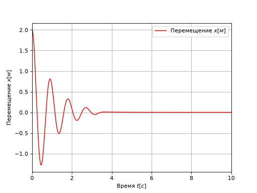
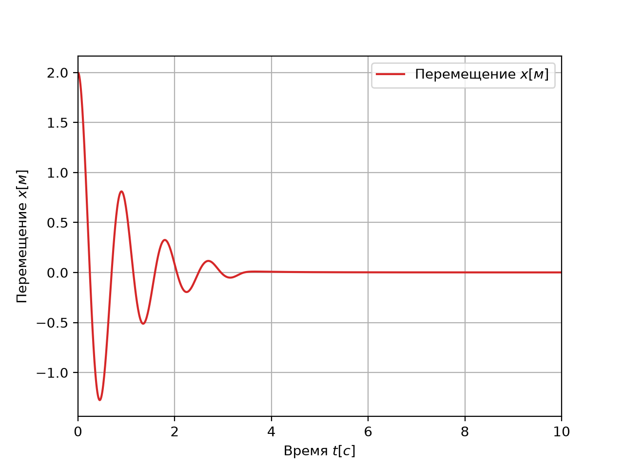
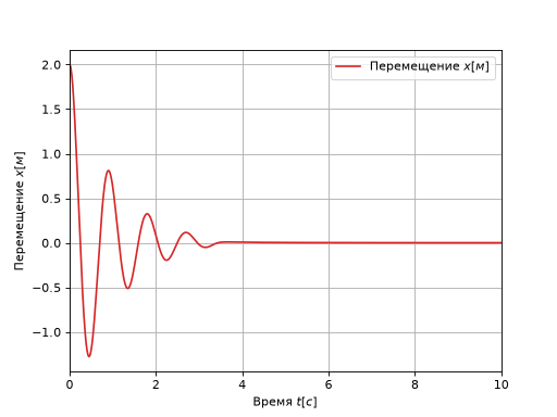
../../../../../_images/plots_plot_pinn_results.png — Results of the PINN model calculation for approximating the equation of displacements of the point mass during damped oscillations#

After loading the model onto the REPEAT VISION platform, the PINN model will be called, and the quality of the approximation results for the solution of the damped oscillation equation of the point mass will be evaluated.

4. Exporting the model to the ONNX format#

The REPEAT VISION platform uses double-precision floating-point values during modeling. Therefore, after training, the model is converted to double-precision mode using the double() method.

5. Creating a project on the REPEAT VISION platform#

First, create a new project and assign it a name, for example, Oscillation Equation Solution.

Next, configure the Simulation time by assigning the corresponding project parameter the value of 10 [s], in accordance with the previously used simulation time for the oscillation process.

Time_of_modeling — Fig. 1 Simulation time#

5.1. Integrating the PINN model into the REPEAT VISION project#

Proceed to create a simple scheme by opening the External Models library. Drag the Approximation Model block onto the project workspace. The block initialization window will automatically open, prompting you to select the corresponding .onnx file.

Block_init — Fig. 2 Initialization of the Approximation Model block#

In the file explorer window, select the previously created model file. The model will then be automatically loaded and initialized.

Init_done — Fig. 3 Model initialization completed#

As seen, after specifying the model file, the block determined the number of input and output ports.

Inputs_and_outputs — Fig. 4 Input and output ports#

In our case, the input port is time, so we will pass the simulation time value to it using the Simulation Time block from the Simulation library. Connect the blocks together.

To obtain the output value of the model, we will use the block Output port from the library External models. Thus, the final diagram looks like this:

OutPort — Fig. 6 Adding the Output port block#

Let’s set up the visualization. To do this, create a chart in the Visualization section with the following parameters:

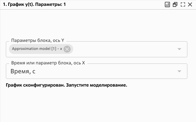
Plot_creation — Fig. 7 Creating a graph#

5.2. Creating a Jython block for analytical solution#

To compare the solution obtained using the neural network, we will use the block Jython. It also needs to be added to the workspace and then click the Edit block code button.

Next, in the code editor of the Jython block, you need to go to the Initialization tab.

As part of the initialization, the parameters of the problem are determined and a function is implemented to obtain an analytical solution to the oscillation equation under consideration.

Initialization#

import math

# Параметры системы
m = 1.0 # масса [кг]
k = 50.0 # жесткость пружины [Н/м]
r = 2.0  # коэффициент демпфирования [Н·с/м]
x_0 = 2.0 # начальное смещение [м]
v_0 = 0.0 # начальная скорость [м/c]

# Вычисляем безразмерные параметры
gamma = r / (2 * m) # коэффициент затухания
omega_0 = math.sqrt(k / m) # собственная частота
omega_1 = math.sqrt(omega_0**1 - gamma**2) # частота затухающих колебаний

def analytical_solution(t):
    """
    Функция выполняет расчёт значения координаты смещения по аналитическому решению уравнения колебаний.

    Параметры:
        t: float
        Текущий момент времени, в который необходимо узнать координату смещения.
    
    Возвращает:
        x: float
        Координата смещения, полученная по аналитической формуле.
    """
    x = (x_0 * math.exp(-gamma * t) * math.cos(omega_1 * t) 
        + (v_0 + gamma * x_0) / omega_1 * math.exp(-gamma * t) * math.sin(omega_1 * t))
    
    return x

Next, in the code editor of the Jython block, you need to go to the Calculation code tab to execute the program at the modeling stage.

As part of the modeling stage, the displacement coordinate is calculated at each time step of the solution.

Calculation code#

# Выполняется расчёт координаты смещения
out_1 = analytical_solution(in_1)

By analogy with the Approximation model block, we add the Simulation time and Output port blocks as input and output, respectively. As a result, the circuit will look like this:

Schema — Fig. 9 Final view of the diagram#

Let’s add a new parameter out_1 of the created Jython block to the previously created graph. To do this, you need to click the Edit button and add a new parameter.

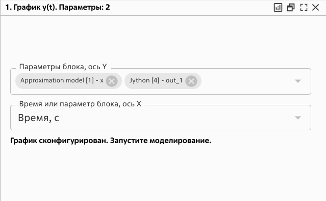
Plot_edit — Fig. 10 Adding the Jython block output to the chart#

5.3. Start calculation, compare results#

Run the calculation by pressing the button Run simulation . The calculation should complete successfully with the following message:

Calculation stopped by solver. Model time limit reached.

In the visualization tab, a graph should be built on which the predicted values of the system displacement coordinate obtained from the approximation model and the analytical values obtained from the Jython block will be displayed in one axes.

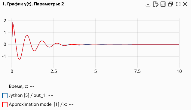
Results — Fig. 11 Graph of calculation results#

6. Conclusions#

During this tutorial you will:

Learned to build a PINN architecture for modeling oscillation dynamics.
Defined a loss function accounting for initial conditions and physical equations.
Trained the model using PyTorch.
Exported the model to ONNX format and added metadata for integration.
Explored the process of integrating the model into the REPEAT VISION platform.
Compared the obtained solution with the analytical one.