

Modeling a DC motor using blocks from the “Automation” section#
The direct current motor (DC motor) is widely used in industry due to the ease of speed control. To analyze its behavior when the supply voltage changes, it is necessary to construct a mathematical model that takes into account electrical and mechanical processes.
In this tutorial, we develop a dynamic model of a DC motor using transfer functions. Instead of explicitly specifying resistance, inductance, and moment of inertia, we will represent the motor as a structural diagram of typical dynamic links:
inertial link (aperiodic) - describes the electrical circuit of the anchor;
integrating link - describes the mechanical part (accumulation of angular velocity under the action of the resulting moment).
This approach (modeling through transfer functions) is standard for automatic control systems. Transfer functions are widely used to analyze linear automatic control systems and allow one to study the dynamics and stability of the system.
1. Statement of the problem#
A model of an object based on physical laws is most often a system of differential equations of the first and second order.
The dynamic behavior of a DC motor with concentrated inertia is described by the following equations:
The electrical equilibrium equation of the armature circuit (1) :
where:
\(U\) – voltage on the armature winding of the motor, [V];
\(E\) – electromotive force (EMF) of the anchor, [V];
\(R\) – armature winding resistance, [Ohm];
\(i\) – armature current, [Ohm];
\(L\) – inductance of the armature circuit, [H];
\(K_e\) – counter-EMF coefficient, [V\(\cdot \frac{rad}{s}\)];
\(\omega\) – engine shaft rotation speed, [\(\frac{rad}{s}\)].
Equation of motion of the motor (2):
where:
\(M\) – electromagnetic torque of the engine, [N\(\cdot\)m];
\(M_c\) – moment of resistance to movement, [N\(\cdot\)m];
\(J\) – total moment of inertia of the anchor and load, [kg\(\cdot\)m\(^2\)];
\(K_M\) – coefficient of electromagnetic moment, [\(\frac{N\cdot m}{A}\)].
In this model, the input effects are the armature voltage \(U\) and the moment of resistance to movement \(M_c\), the output variables are the electromagnetic torque of the motor \(M\) and the rotation frequency of the motor shaft \(\omega\).
It should be noted that some manufacturers do not specify the \(K_e\) coefficient in the technical parameters of the DC motor model. In this case, manual calculations must be performed using (3) :
To construct a model in the form of a structural diagram, the Laplace transform is performed.
The Laplace transform allows us to move from differential equations to algebraic expressions—transfer functions. This significantly simplifies the analysis and construction of control system structural diagrams.
DC motor consists of two main parts: electromagnetic and electromechanical parts.
The transfer function of the electric circuit is described by a first-order aperiodic link (4) :
where:
\(s\) - Laplace operator;
\(T_{em} = \frac{L}{R}\) is the time constant describing the dynamics of electromagnetic processes in DC motor.
The inductance of the armature circuit prevents an instantaneous change in current, therefore the electrical part of the motor has inertia and is described by a first-order aperiodic link.
The mechanical part of the engine has integrating properties and is described by the integrating link (5):
where \(K_m\) is the coefficient of electromagnetic moment.
The integrating link reflects the fact that the angular velocity of the engine accumulates over time under the action of the resulting torque.
2. Creating and setting up a project#
First you need to create a new project and give it a name, for example, DC Motor.
Then you need to make the following project settings (see Fig. 1 below):
Disable the
Synchronization with real timeoption;Set the
Simulation timeparameter to 1 [s];Set the
Integration stepparameter to 1 [ms];Set the
Sampling stepparameter to 1 [ms].
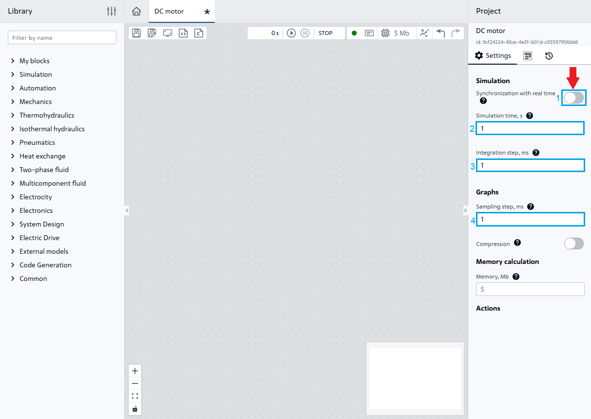
Fig. 1 Project setup#
3. Development of a DC motor model#
As an example, a DC motor is being developed with the following technical parameters:
rated power \(P_{nom}\) = 0.37 [kW];
voltage at the motor input \(U_{nom}\) = 110 [V];
nominal angular velocity \(\omega_{nom}\) = 314.16 [\(\frac{rad}{s}\)];
armature resistance \(R_{nom}\) = 0.546 [Ohm];
armature current \(I_a\) = 4.4 [A];
armature inductance \(L_{nom}\) = 2.2 [mH];
coefficient of electromagnetic moment \(K_m\) = 0.27 [\(\frac{N\cdot m}{A}\)];
moment of inertia of the shaft \(J\) = 0.00408 [kg\(\cdot\) m\(^2\)].
According to the formula (3), the back-EMF coefficient is calculated. \(K_e=0.34 [\frac{V \cdot s}{rad}]\)
Other coefficients and parameters of the dynamic model DC motor (6) :
Let’s add the following blocks of the Automation library to the canvas, assigning them property values according to the previously performed calculations:
Two Constant blocks (voltage \(U_{nom}\) = 100 [V], load torque \(M_{load}\)=1.2 [N\(\cdot\) m]), assigning the
Constant valueproperty for the first block the value110, and for the second block the value1.2;Two blocks Signal difference (Controller error) (Consider feedback on EMF);
Inertia block (Electromagnetic part: \(\frac{\frac{1}{R_я}}{T_{em} \cdot s +1}\)), assigning the following values to the properties:
Property |
Value |
|---|---|
Gain |
|
Characteristic time |
Integrating block (Time domain integration) (Mechanical part: \(\frac{K_m}{s \cdot J}\)), assigning the property
Gainthe value66.167;Branching (To create a feedback loop for EMF), assigning the
Number of output portsproperty the value2;Two Gain blocks (For the coefficients \(\frac{1}{K_m}\) and \(K_e\)), assigning the
Gainproperty for the first block the value0.34, and for the second block the value3.7.
Important
In REPEAT VISION decimal numbers are separated by a dot.
Then you need to connect the blocks according to Fig. 2:
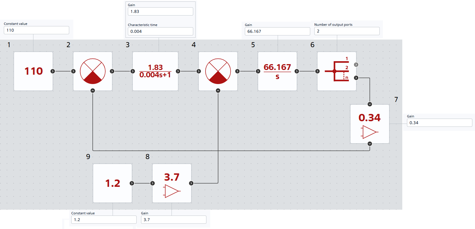
Fig. 2 Connection of blocks#
To improve the readability of the diagram, we will assign the Block label property to the blocks, Fig. 3:
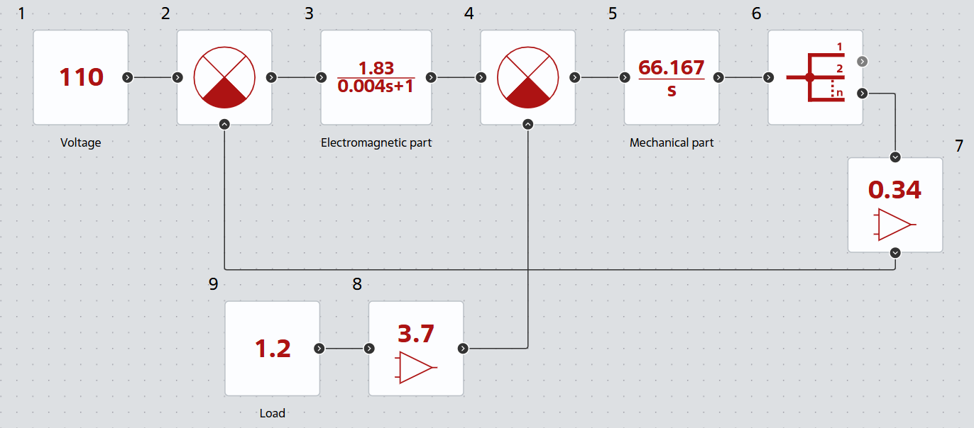
Fig. 3 Adding labels to blocks#
The model is ready for calculation. The general diagram with transfer functions and coefficients is shown in Fig. 4:
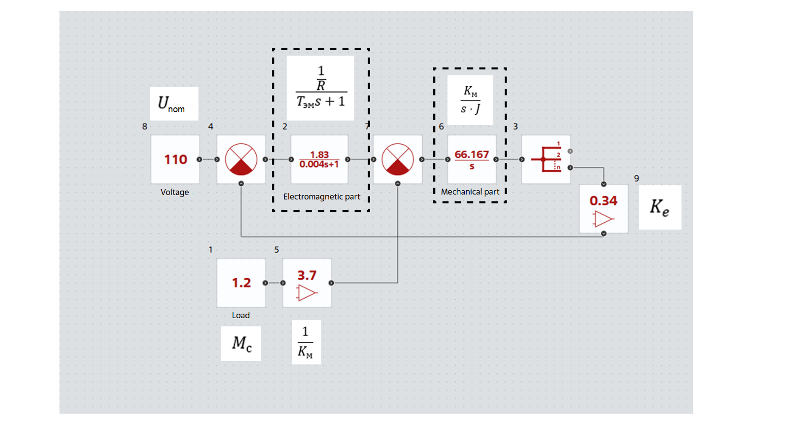
Fig. 4 General diagram of the model#
4. Analysis of calculation results#
Next, the model is calculated and the controlled parameter is analyzed (shaft angular velocity, block Branching). The graphs of the output angular velocity \(\omega\) of the shaft of a DC motor are shown in Fig. 5:
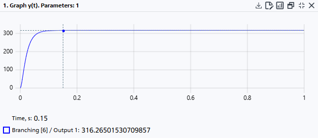
Fig. 5 Graph of the angular velocity of the shaft#
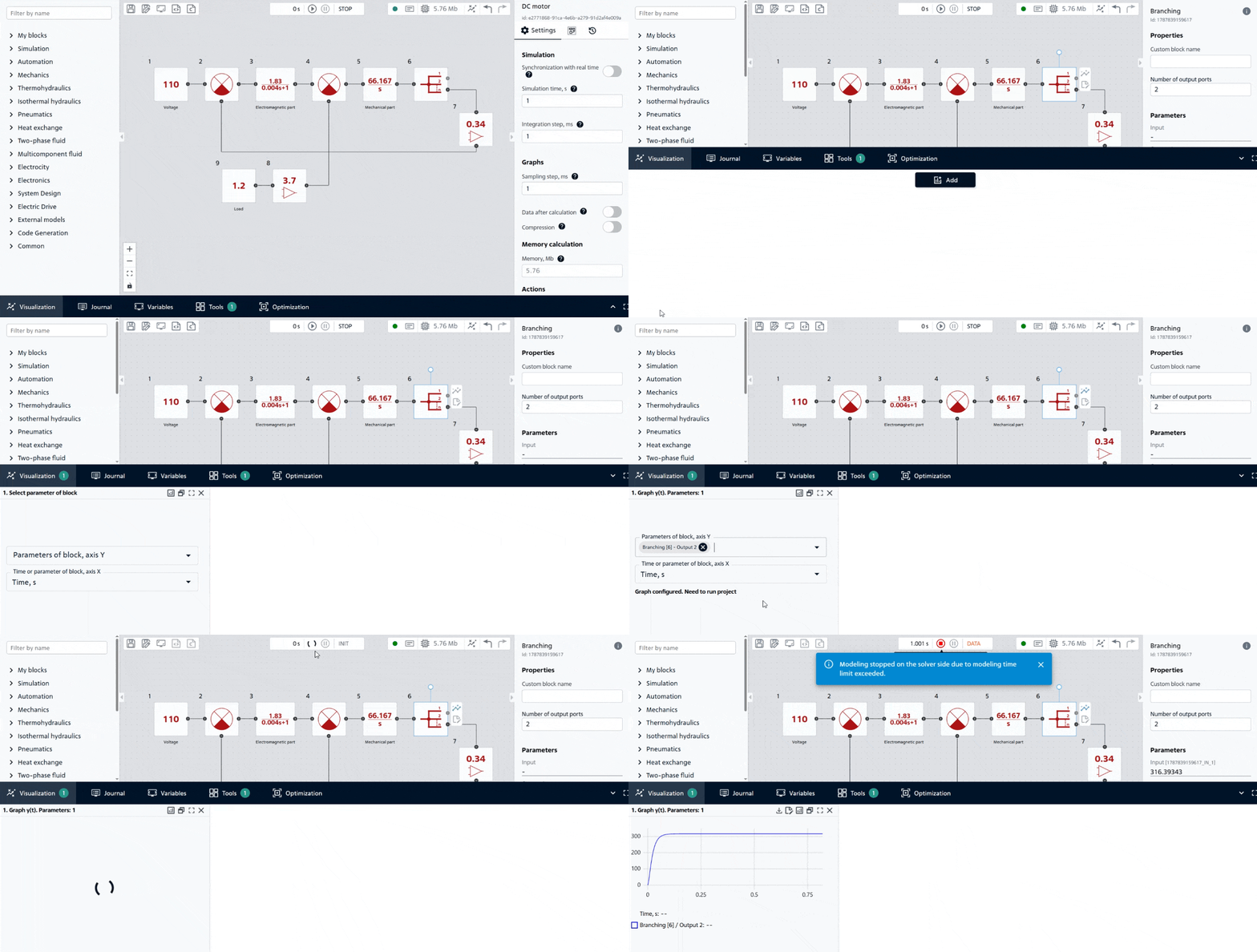
Fig. 6 Adding a graph and starting the calculation#
The angular velocity of the motor increases gradually because the armature current and the mechanical system have inertia. Additionally, an increase in speed causes an increase in the back-EMF, which reduces the motor current.
The relative control error \(\delta\) (an indicator of process accuracy) is determined using the formula (7):
The nominal value of the angular velocity \(\omega_{nom}\)=314.16 \(\frac{rad}{s}\) and differs slightly from the simulation results \(\omega_{ust}\)=316.26, which indicates the successful development of the model.
5. Modification of the circuit#
The constructed model of the DC motor allows for easy connection of various signal sources and signal transformation. This demonstrates the flexibility of structured modeling using Automation blocks. Consider two simple additions:
Conversion of angular velocity to rotational speed (rpm).
Create another Gain block and connect it to a free output port of the Branching block. Since REPEAT VISION supports arithmetic expressions in block properties, assign the new amplifier the value 60/(2*pi), Fig. 7:
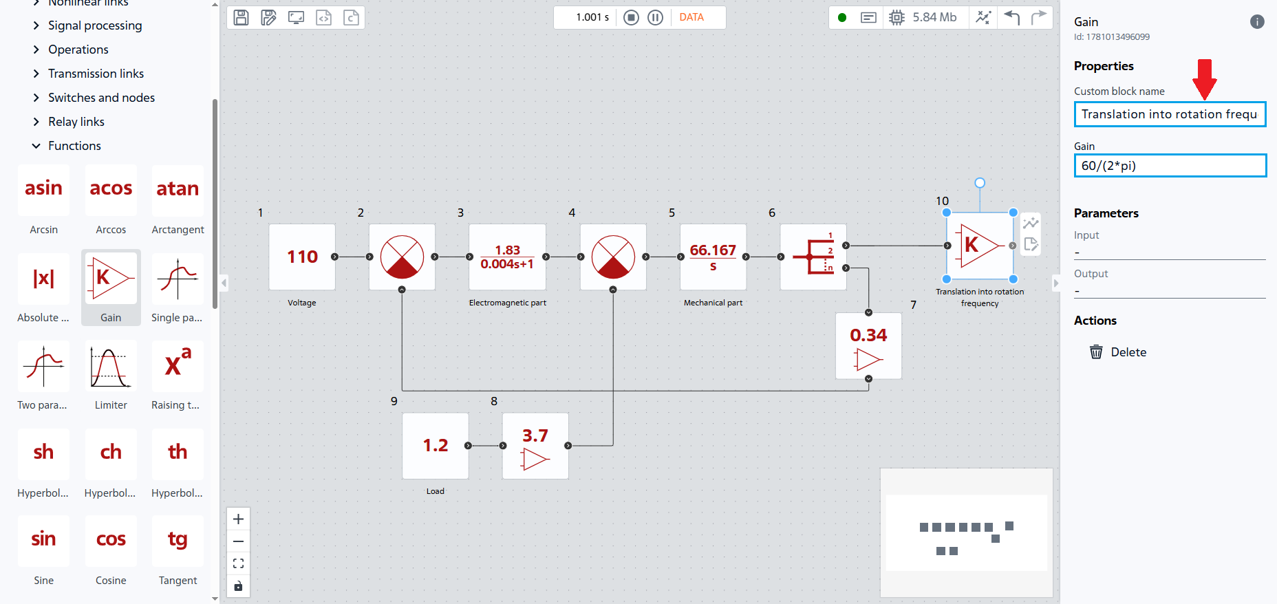
Fig. 7 Conversion of angular velocity into rotation frequency#
Теперь мы имеем в модели параметр угловой частоты: \(316.26 \frac{рад}{с}=3021.335 \frac{об}{мин}\).
Conversion of units of measurement allows the results of modeling to be presented in a more familiar engineering form.
Dynamic load moment.
Let’s add the dynamics of load change (see Fig. 8 below), for this replace the Constant block, which defines the load \(M_c\) with the Piecewise constant function block, assigning it the following property values:
Property |
Value |
|---|---|
Vector of time arguments, s |
|
Vector of function values |
1.2;2.4 - which corresponds to a doubling of the load at t = 0.5 s. This will allow us to see how the speed responds to an increase in external disturbance |
Periodicity |
Off |
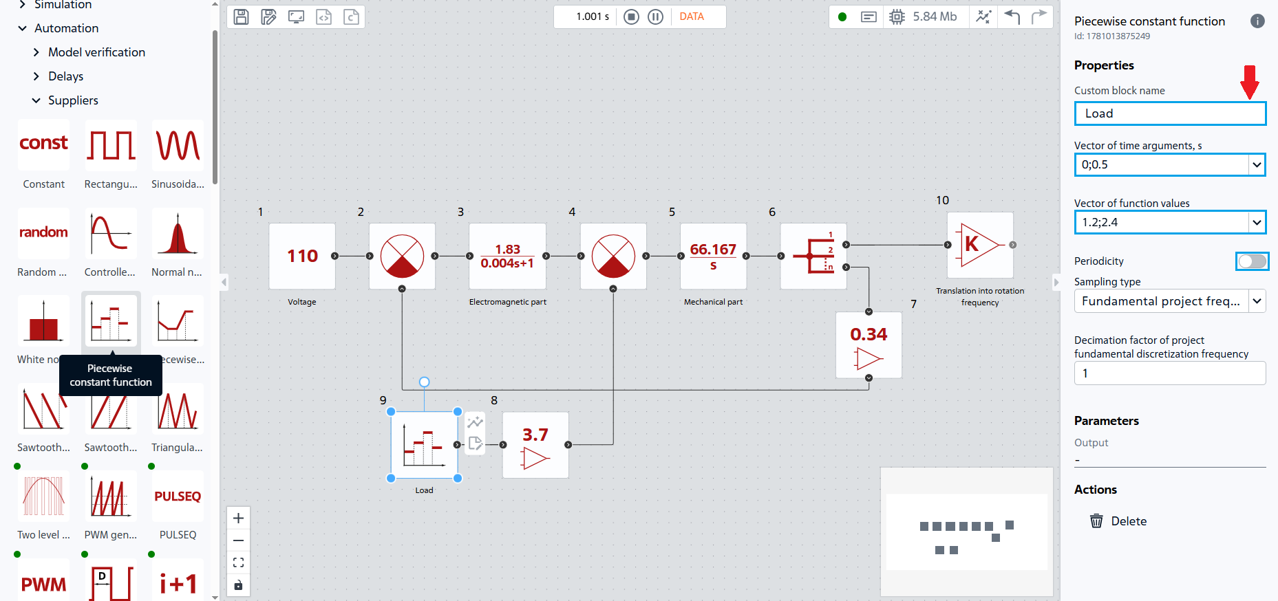
Fig. 8. Model of a DC motor with dynamic load#
After re-calculating with a dynamic load, having studied the angular velocity graph, we can conclude that with an increase in load to 2.4 [N\(\cdot\)m] there was a drop to 309.26 [\(\frac{rad}{s}\)], Fig. 9:
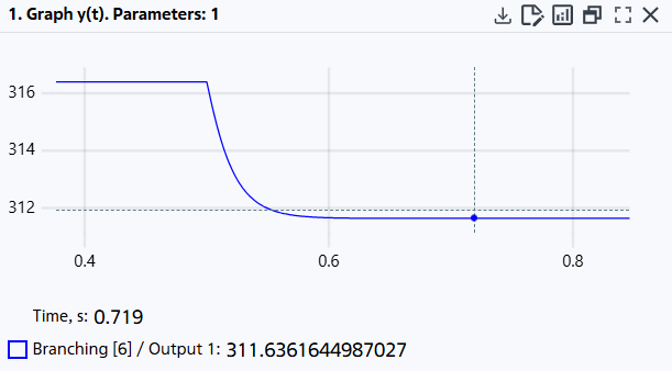
Fig. 9. Decrease in angular velocity with increasing load#
An increase in the load torque results in a decrease in the steady-state speed of the motor, since the counteracting mechanical torque on the shaft increases.
6. Conclusion#
This tutorial covers:
Transformation of differential equations describing physical processes in DC motor into the form of transfer functions;
Development of a DC motor model using blocks from the Automation section with calculation of parameters based on passport data;
Model accuracy check: the discrepancy between the established speed and the nominal speed was 0.67%;
Modification of the circuit: conversion of the signal unit (block Gain) and creation of a dynamic load (block Piecewise constant function).