Implementing a moving average filter using a Java-function block

Note

The model built in this tutorial is available in demo projects: Filter “Moving average” – Java function.

 In the real world, data is rarely perfect. Controlled parameters often contain random noise that must be “filtered out” and ignored. This tutorial describes the steps for developing a «Moving average» filter using the Java-function block.

 In many control systems, measurement filtering helps improve stability and reduce the impact of noise. In automatic control systems, a “raw” noisy signal can lead to a number of negative consequences:

• Wear of actuators: constant high-frequency vibrations cause actuators (motors, valves, relays) to perform micro-movements, which leads to their premature failure.

• False protection alarms: a random noise spike may be mistakenly identified by the system as an emergency, leading to an unjustified shutdown of the equipment.

• Control loop instability: noise wreaks havoc on the operation of controllers (e.g., PID controller), causing self-oscillations and reducing the accuracy of maintaining set parameters.

 The tutorial covers:

• Logic for working with arrays: creating a data buffer and implementing a “ring queue” algorithm for storing signal history.

• Mathematical processing: Real-time arithmetic mean calculation to suppress high-frequency noise.

• Mathematical processing: Real-time arithmetic mean calculation to suppress high-frequency noise.

• The org.apache.commons approach: Optimizing code using the Apache Commons Math standard library to improve robustness and make coding easier to write.

 Advantages of using the Java function for this task:

• Algorithm extensibility: Using the Java language allows you to extend the basic filtering with arbitrary logic, such as input data validation, exception handling, or the implementation of non-linear processing algorithms.

• Integration of external solutions: The ability to import third-party Java packages provides access to verified mathematical libraries, which reduces development time and minimizes the likelihood of software errors.

• Conciseness and readability of the model: Implementing complex mathematical algorithms or multi-level logical conditions within a Java function allows you to avoid creating cumbersome and difficult-to-read diagrams from hundreds of standard blocks. A single compact text block replaces entire subsystems, simplifying the visual structure of the model and facilitating its further debugging and maintenance.

1.  Statement of the problem

 During the simulation, a signal with Gaussian noise is fed to the input of the Java-function.

 The goal of this tutorial is to develop a user-defined function that smooths an input signal by calculating its arithmetic mean within a sliding time window of fixed length.

 To store the signal history, an array (buffer) of n elements is created, where n is the filtering depth (window size). At each calculation step k, the algorithm performs the following operations:

1. Updating the data array: adding the current value \(x_k\) and removing the oldest value \(x_{k-n}\).

2. Calculation of the output smoothed value \(y_k\) using the simple moving average formula (1):

(1)\[y_k=\frac{1}{n}\cdot \sum^{n-1}_{i=0}x_{k-i}\]

where:

 \(y_k\) - filtered value of the signal at the current step;

 \(x_{k-i}\) - current and previous values ​​of the input signal stored in the array;

 \(n\) - the number of calculation points in the smoothing window (array size).

2.  Creating and setting up a project

 First you need to create a new project and give it a name, for example, Moving Average - Java-function.

 Then you need to make the following project settings (see Fig. 1 below):

1. Disable the Synchronization with real time option;

2. Set the Simulation time parameter to 10 [s];

3. Set the Integration step parameter to 10 [ms];

4. Set the Sampling step parameter to 10 [ms].

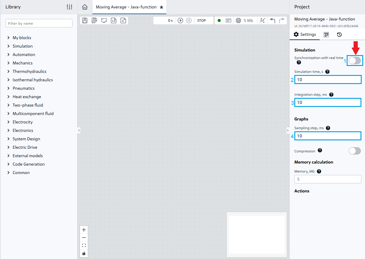
Fig. 1 Project setup

3.  Creating a Signal Source

 First of all, it is necessary to develop a signal source with noise. To do this, it is necessary to add the following blocks to the canvas:

• Normal noise, located in the Automation library, in the Suppliers section, with the following property values ​​set (see Fig. 2 below):

Property	Value
Custom block name	Signal with noise
Expected value	45
Standard deviation	5
Sampling period, s	0.01

• Piecewise constant function, located in the Automation library, in the Suppliers section, with the following property values ​​set (see Fig. 2 below):

Property	Value
Custom block name	Piecewise change of signal at time t = 5 s
Vector of time arguments, s	0;5
Vector of function values	0;15
Periodicity	Off

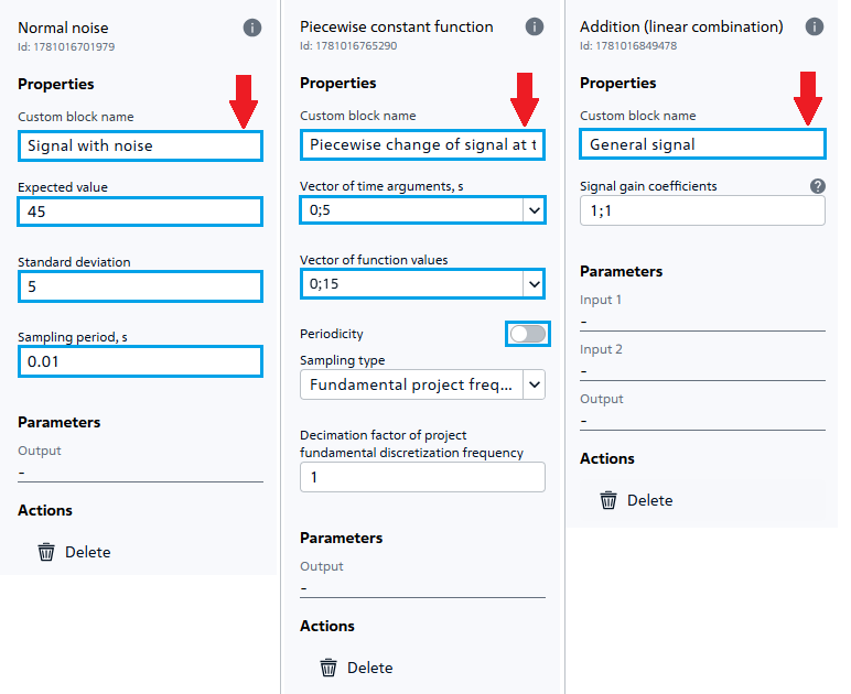
Fig. 2 Setting properties for signal source blocks

• Addition (linear combination), located in the library Automation, section Operations.

Note

The block properties remain default, you only need to add Block label - Common signal

 These blocks must be connected to each other according to Fig. 3:

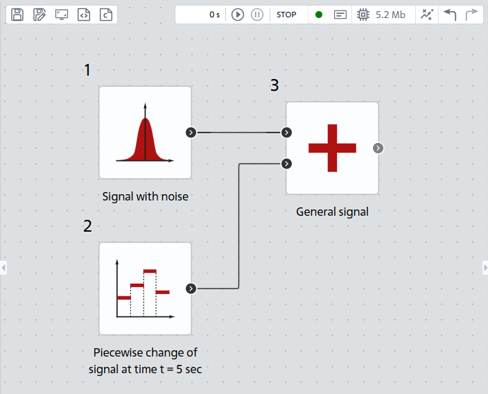
Fig. 3 Connecting blocks

 As a result, we have a noisy signal source whose amplitude dynamically changes at time t = 5 [s]. Next, to conduct a test calculation of the model, it is necessary (see Fig. 4 below):

1. Select the Addition (linear combination) block by clicking on it with LMB;

2. Open the Visualization tab located in the bottom left panel and click LMB the Add button;

3. In the window that opens, select the output value of the block Addition (linear combination);

4. Run the calculation with the button Run the simulation.

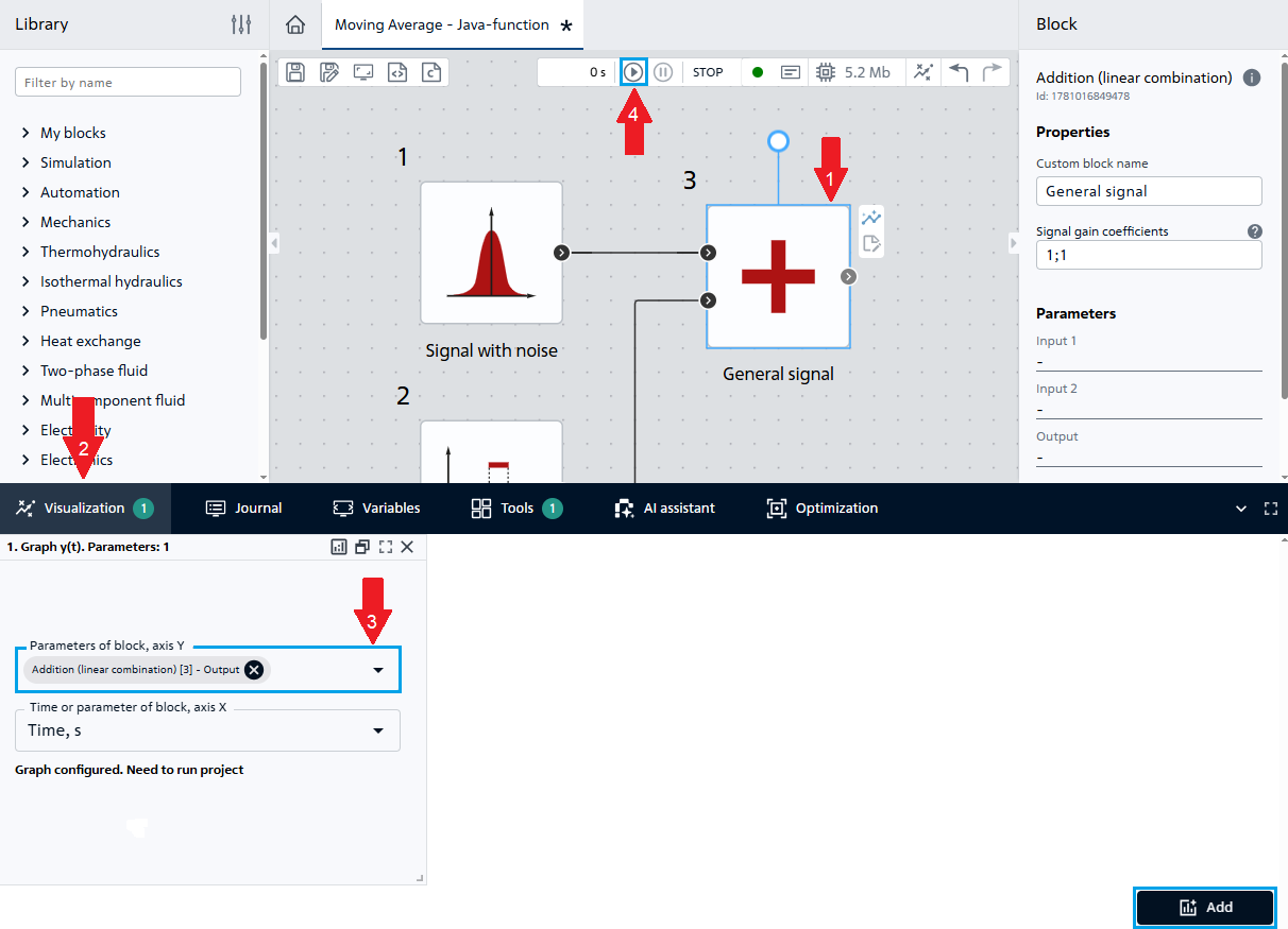
Fig. 4 Preparation for calculation

 After the calculation is completed, a noisy signal will be obtained (see Fig. 5 below), which must be smoothed using the “Moving average” algorithm, implemented in the Java function.

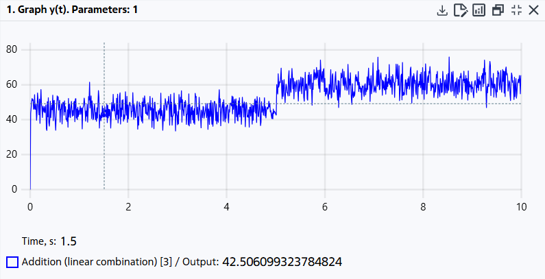
Fig. 5. Signal-to-noise graph

4.  Java function for implementing the “Moving average” filter

 The Java-function block (see Figure 6 below) from the External models section is a programmable component that allows you to embed custom Java code into the overall modeling scheme. The logic of the block is described in the built-in editor, which is opened by double-clicking LMB (see Fig. 7 below), which makes it possible to implement algorithms of any complexity.

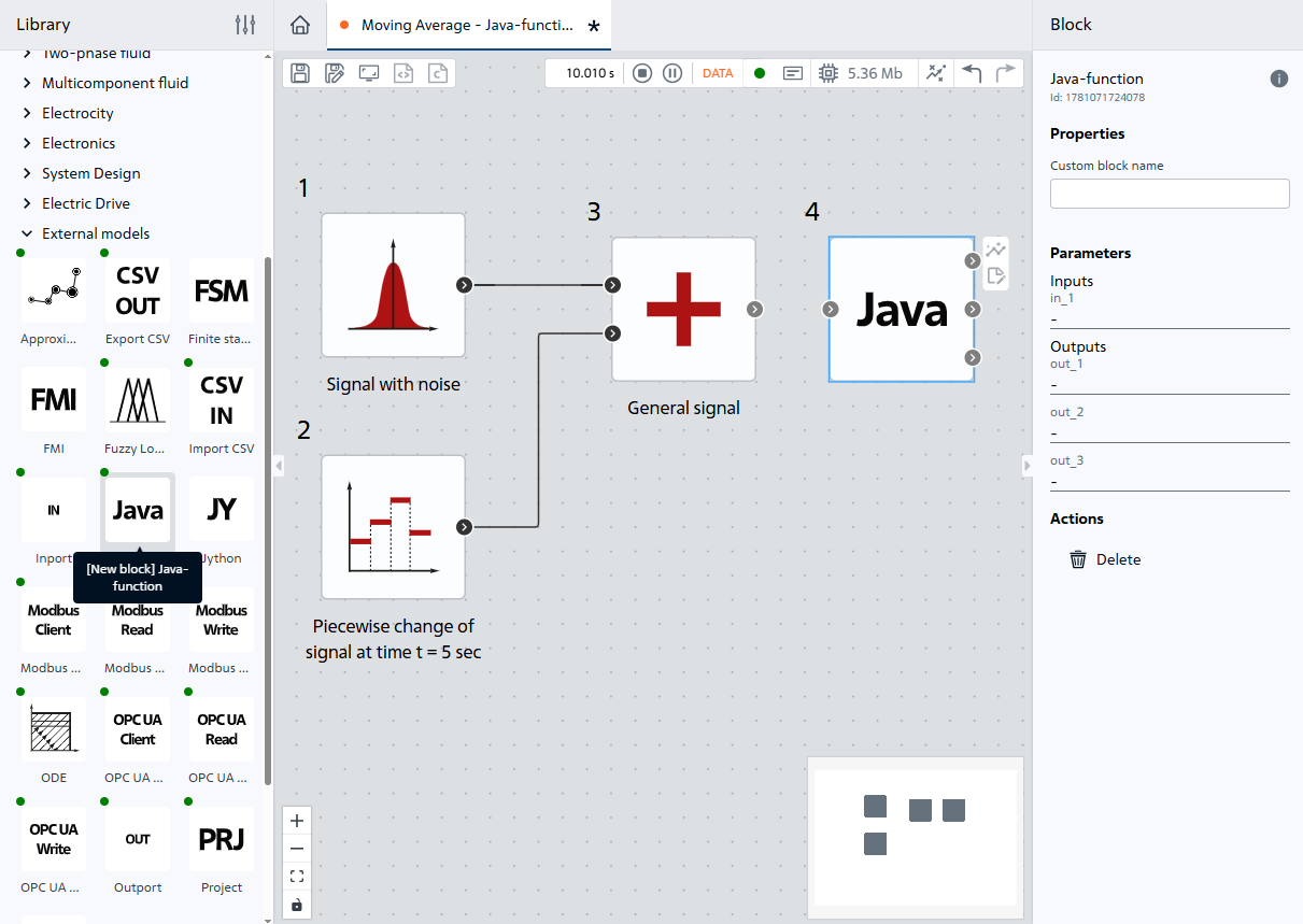
Fig. 6 Java-function block

Fig. 7 Java block editor

 The block contains four subsections with code:

• Import – for importing Java libraries (for example: import java.lang.Math;);

• Initialization – for declaring and initializing global variables;

• Modeling code – the main calculation code in which calculation methods are called;

• Methods – for writing custom methods.

 The block also has configurable input and output ports: in_1 (input) and out_1, out_2, out_3 (output) by default.

 Before implementing your own code to apply a smoothing filter, you must:

1. Clear each subsection, Fig. 8:

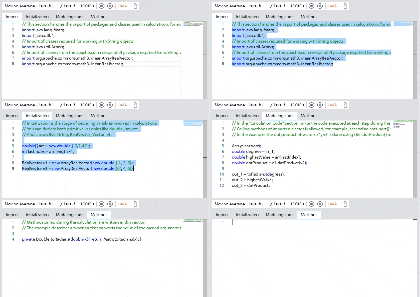
Fig. 8 Empty editor tabs

2. Change the number of output ports to one by clicking on the red button -, located in the right panel next to each port name and appearing when you hover the cursor over the desired parameter, Fig. 9:

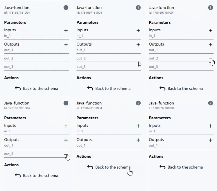
Fig. 9 Removing the block output port

 As a result, before writing the smoothing filter code, the custom Java function will have one input and one output port and empty subsections.

 Let’s connect the block according to the general diagram of the model, Fig. 10:

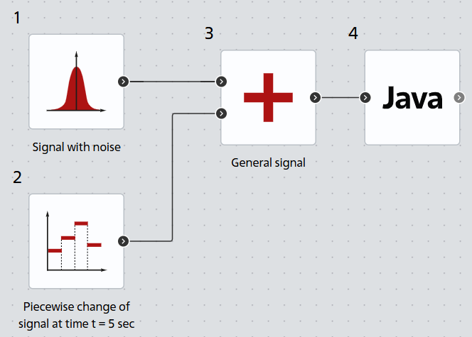
Fig. 10 General diagram of the model

 The following is the code used to implement the smoothing filter according to subsections. Comments are delimited by // characters.

4.1.  Imports

 This section imports packages and classes used in calculations, for example, the java.lang.Math class, which contains mathematical functions.

import java.lang.Math;
import java.util.*;
import java.util.Arrays;

• Line 3. Importing classes needed to work with arrays

4.2.  Initialization

int windowSize = 20;
double[] buffer = new double[windowSize];
int currentIndex = 0;
boolean bufferFull = false;

• Line 1. To allocate memory for the array (buffer), an integer variable named windowSize must be created. A value of 20 means the filter stores the last 20 samples.

• Line 2 By default, all elements of type double in Java are initialized to 0.0.

• Line 3. A pointer to the current array cell where the new input value will be written. Indexing in Java starts at 0, so the starting position is 0.

• Line 4. Marker flag. Set to true when the array is completely filled with the first 20 values. This is necessary for the correct calculation of the average value at the initial stage of the simulation.

4.3.  Modeling code

 Occurs at each step of the model. Here, the processSignal(in_1) method is called, the signal value with noise in_1 is passed, and the result is written to the output port out_1.

out_1 = processSignal(in_1);

• Line 1. The “Modeling code” contains the code executed at each step of the model calculation; in our case, it’s a call to the smoothing filter method. out_1 is the block’s output port (the smoothed signal value). in_1 is the input port (the signal value with noise).

4.4.  Methods

 The filter logic itself is located here. The processSignal() method is written, which updates the ring buffer and returns the moving average.

public double processSignal(double rawSignal) {
   buffer[currentIndex] = rawSignal;
   currentIndex++;
   if (currentIndex >= buffer.length) {
    currentIndex = 0;
    bufferFull = true;
    }
    double sum = 0.0;
    int count = bufferFull ? buffer.length : currentIndex;
    for (int i = 0; i < count; i++) {
        sum += buffer[i];
        }
        return sum / count;
        }

• Line 2. STEP 1: Write new data to the circular queue (ring buffer). Place the current noisy sensor value in the cell with the index currentIndex.

• Line 3. STEP 2: Index management and buffer overflow control. Advance the pointer to the next cell for the next simulation step.

• Line 4. We check if we’ve exceeded the array’s bounds (going out of bounds will cause an error). The buffer.length property dynamically returns the array’s size (in this case, 20).

• Line 5. Reset the index to 0. New data will begin to overwrite the oldest data.

• Line 6. We set the flag: the buffer is full, now all 20 cells contain real data.

• Line 8. STEP 3: Calculate the moving average. Local variable for accumulating the sum. Reset to 0 at each step.

• Line 9. We set the number of elements to calculate the average. If the buffer is full (bufferFull == true), we divide by the array length (20). If the buffer is still filling, we divide only by the number of elements actually written (currentIndex).

• Line 10. We start a loop to iterate over the array elements and sum them. The variable ‘i’ is the loop counter, which is incremented by 1 (i++) on each iteration. The loop continues as long as ‘i’ is strictly less than ‘count’.

• Line 11. Accumulate the sum: sum = sum + buffer[i].

• Line 13. Return the calculation result. Dividing the sum by the number of elements yields the final filtered value.

The code for implementing the “Moving average” filter in a Java function has been written.

4.5.  Analysis of calculation results

 To evaluate the filter’s performance and perform a comparative analysis of the filtered signal, we will add a second parameter to the graph: “Java function – out_1”, Fig. 11:

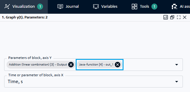
Fig. 11 Adding a Java block output port graph

 According to the obtained graphs (see Fig. 12 below), it can be concluded that the moving average suppresses high-frequency noise, since random positive and negative deviations partially compensate each other when averaging. At the same time, the slowly changing useful component of the signal is preserved.

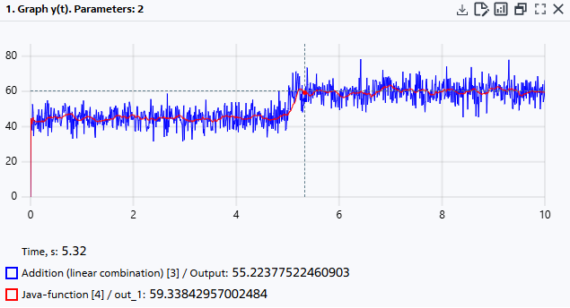
Fig. 12 Signal with noise and filtered signal

 Next, the calculation is performed with a sampling window equal to 100. For this, the value of the windowSize variable is set to 100.

int windowSize = 100;
double[] buffer = new double[windowSize];

• Line 2 By default, all elements of type double in Java are initialized to 0.0.

 When increasing the size of the filter window, you will notice:

1. Significant improvement in signal smoothing and noise suppression;

2. The appearance of a time delay in the output signal relative to the input signal.

 The delay occurs because the filter’s output value is calculated as the average of the last few signal samples. The larger the window size, the more noise is suppressed, but the slower the filter responds to rapid changes in the input signal.

 With a sampling step of 10 [ms] and a window size of 100 samples, the filter averages the values ​​over a time interval of about 1 [s], so the change in the output signal occurs noticeably slower compared to the original signal, Fig. 13:

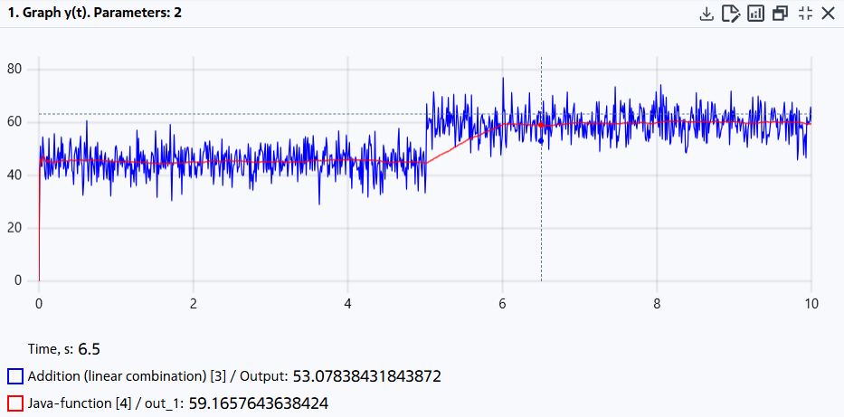
Fig. 13 Results of the filter with an enlarged window

5.  Implementing a Filter Using Apache Commons Math

 A manually implemented moving average filter is fully functional, but in real-world projects, it’s often more advantageous to use standard mathematical libraries. This reduces development time, reduces the likelihood of errors, and provides access to additional statistical methods.

 One of the most popular Java libraries for numerical computations is Apache Commons Math. In our case, the DescriptiveStatistics class automatically implements a circular buffer, calculating the mean, variance, median, and other statistics.

 Below is the complete code for each section of the Java-function block using the DescriptiveStatistics class from the Apache Commons Math package.

5.1.  Import

 This subsection adds the import of the DescriptiveStatistics class.

 This section imports packages and classes used in calculations, for example, the java.lang.Math class, which contains mathematical functions and constants

import java.lang.Math;
import java.util.*;
import java.util.Arrays;
import org.apache.commons.math3.stat.descriptive.DescriptiveStatistics;

• Line 3. Imports the classes needed to work with String objects.

• Line 4. Importing class DescriptiveStatistics from package org.apache.commons.math3.stat.descriptive.

5.2.  Initialization

 A single DescriptiveStatistics object is created with the specified window size.

int windowSize = 100;
DescriptiveStatistics stats = new DescriptiveStatistics(windowSize);

• Lines 1-2. Create a statistics object with a windowSize of 100 elements.

5.3.  Modeling code

 processSignal(in_1) is still called.

out_1 = processSignal(in_1);

• Line 1. The “Modeling code” contains the code executed at each step of the model calculation; in our case, it’s a call to the smoothing filter method. out_1 is the block’s output port (the smoothed signal value). in_1 is the input port (the signal value with noise).

5.4.  Methods

 The processSignal() method contains only two main lines: add a value and return the average. The library manages the buffer itself.

public double processSignal(double rawSignal) {
    stats.addValue(rawSignal);
    double mean = stats.getMean();
    return mean;
    }

• Line 2. Add a new value. The library will automatically delete the oldest value if the window is full.

• Row 3. We obtain the arithmetic mean.

• Line 4. Bonus: we can easily get the standard deviation (noise). double std = stats.getStandardDeviation();

 Next, a comparison is made between filters created manually and those using the DescriptiveStatistics class.

6.  Comparison of Implementations: Manual Filter and Apache Commons Math

 To check the identical operation of filters of two different designs, we need to duplicate the source of a signal with noise - for this we will need the Branching block (the Automation library, the Switches and nodes section), in which we need to change the value of the Number of output ports property to 2. The connection diagram is shown in Fig. 14:

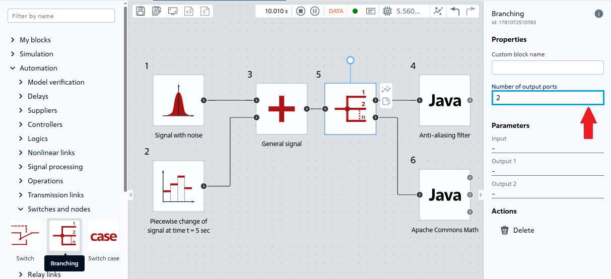
Fig. 14 Adding a splitter to duplicate the signal

 Let’s plot three signals on one chart (see Fig. 15 below):

1. Signal with noise;

2. Filtered signal from a hand-written filter;

3. Filtered signal from a filter implemented using the DescriptiveStatistics class.

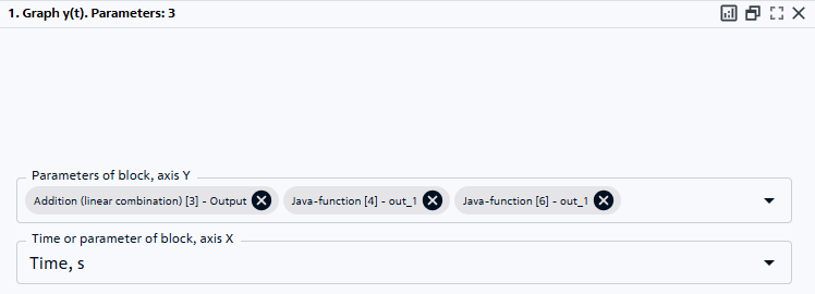
Fig. 15 Parameters for plotting a graph

 The results of the smoothed signal values ​​coincide with high accuracy, Fig. 16:

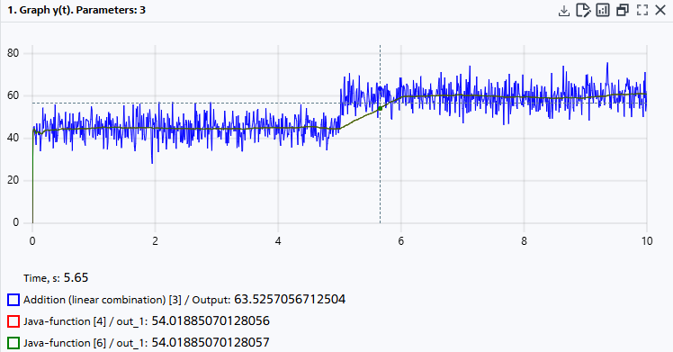
Fig. 16 Results of two filters

 The DescriptiveStatistics class isn’t the only useful component of the Apache Commons Math library. It includes modules for solving other mathematical problems:

• linear - operations with matrices and vectors, solving systems of linear equations;

• analysis - numerical solution of equations, interpolation, integration;

• random - generation of random numbers with different distributions;

• stat - additional statistical methods (regression, tests).

Note

A detailed description of all modules is available on the official website

7.  Conclusion

 This tutorial covers:

1. Implementation of a moving average filter using a ring buffer and manual calculation of the arithmetic mean using the Java-function;

2. Using the Apache Commons Math external library in the Java-function block to import the DescriptiveStatistics class, which automatically manages the data window and returns the mean;

3. The influence of the filtering window size on the smoothing quality and signal delay: increasing the window improves noise suppression, but increases the time delay;

4. Comparison of two implementations – their results are identical, which confirms the correctness of the written algorithm.