

Sequential and parallel operation of pumps#
1. Introduction#
In engineering, whether designing water supply systems, aircraft fuel systems, or industrial process lines, pumps rarely operate alone. To achieve the required parameters—higher pressure or higher flow—engineers combine pumps to operate together.
This raises a number of questions: How can we predict the behavior of such a system before its physical assembly? How can we avoid costly errors and find the optimal configuration? The answer lies in the use of system modeling and calculations.
In this tutorial, we will focus on two fundamental ways of connecting pumps: series and parallel. Using the REPEAT VISION environment, we will learn how to create, configure, and analyze virtual models of these systems. You will see how changing the configuration directly impacts the key output parameters: flow rate (Q) and head (H).
2. The model in question and its characteristics#
This tutorial examines the network and pump model presented in the tutorial Construction of the flow-pressure characteristic of the network (see Fig. 1 below).
The process of building a model and filling in the properties is shown in the tutorial.
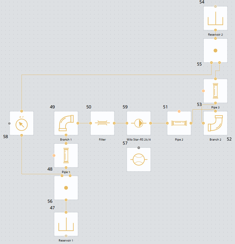
Fig. 1 Model of a hydraulic network with a Wilo Star-RS 25/4 pump#
Let’s plot the pump and network curves based on the data obtained in this tutorial. The code for plotting them is provided below.
Important
Please note that in the context of this tutorial, the relationship between the REPEAT VISION model and JupyterLite is not established. In this case, it is used as a convenient visualization tool.
Construction of pump and network characteristics
# Импорт необходимых библиотек
import piplite
import pandas as pd

# Характеристика сети
system_head_curve_df = pd.DataFrame({
    'massFlowRate': [0.000000, 0.036842, 0.073684, 0.110526, 0.147368, 0.184211,
                     0.221053, 0.257895, 0.294737, 0.331579, 0.368421, 0.405263,
                     0.442105, 0.478947, 0.515789, 0.552632, 0.589474, 0.626316,
                     0.663158, 0.700000],
    'pressureDrop': [30000.000000, 30037.216415, 30171.196080, 30356.192800,
                     30591.674870, 30879.679700, 31218.609300, 31607.275800,
                     32044.753000, 32530.294700, 33063.283000, 33643.198700,
                     34209.597000, 34942.093300, 35660.350000, 36424.071000,
                     37232.990700, 38086.874000, 38985.507000, 39928.697000]
})

# Характеристика насоса Wilo Star-RS 25/4
pump_curve_df = pd.DataFrame({
    'massFlowRate': [0.0, 0.0693, 0.1386, 0.2079, 0.2772, 0.3465, 0.3881],
    'pressureDrop': [38182.5, 36028.6, 33776.8, 31525.0, 29077.4, 26434.0, 24867.6]
})

# Импортируем и устанавливаем необходимые библиотеки для визуализации
import matplotlib.pyplot as plt
await piplite.install("seaborn")
import seaborn as sns

def plot_pressure_drop_curve(system_head_curve_df, pump_curve__df, figsize=(10, 6)):
    """
    Создает график зависимости потерь давления от массового расхода.

    Parameters:
    -----------
    system_head_curve_df : pd.DataFrame
        DataFrame с колонками 'massFlowRate' и 'pressureDrop' для характеристики сети
    pump_curve__df : pd.DataFrame
        DataFrame с колонками 'massFlowRate' и 'pressureDrop' для характеристики насоса
    figsize : tuple
        Размер графика в дюймах (ширина, высота)
    """

    # Настройка стиля графика
    plt.style.use('seaborn-v0_8-dark')

    # Создаем фигуру и оси с указанным размером
    fig, ax = plt.subplots(figsize=figsize, dpi=100)

    # Фильтруем данные, исключая NaN значения для чистоты графика
    clean_data = system_head_curve_df.dropna(subset=['pressureDrop'])
    # Данные для насоса
    clean_pump_data = pump_curve__df.dropna(subset=['pressureDrop'])
    # Проверяем, есть ли данные для отображения
    if len(clean_data) == 0:
        print("Нет данных для построения графика (все значения NaN)")
        return

    # Создаем основной график - линию с маркерами
    # Используем маркеры 'o' для точек и линию для соединения

    # График РНХ сети
    ax.plot(clean_data['massFlowRate'],
            clean_data['pressureDrop'],
            marker='o',                # Маркеры в виде кружков
            markersize=8,              # Размер маркеров
            linewidth=2,               # Толщина линии
            color='steelblue',         # Цвет линии
            alpha=0.8,                 # Прозрачность
            label='Характеристика гидравлической сети',   # Метка для легенды
            markerfacecolor='white',   # Заливка маркеров
            markeredgewidth=2)         # Толщина обводки маркеров

    # График РНХ насоса
    ax.plot(clean_pump_data['massFlowRate'],
            clean_pump_data['pressureDrop'],
            marker='o',                # Маркеры в виде кружков
            markersize=8,              # Размер маркеров
            linewidth=2,               # Толщина линии
            color='#e63946',            # Цвет линии
            alpha=0.8,                 # Прозрачность
            label='Характеристика насоса',   # Метка для легенды
            markerfacecolor='white',   # Заливка маркеров
            markeredgewidth=2)         # Толщина обводки маркеров

    # Настройка осей графика
    ax.set_xlabel('Массовый расход, кг/с',
                  fontsize=12,
                  fontweight='bold',
                  labelpad=10)  # Отступ подписи от оси

    ax.set_ylabel('Потери давления, Па',
                  fontsize=12,
                  fontweight='bold',
                  labelpad=10)  # Отступ подписи от оси

    # Заголовок графика
    ax.set_title('Расходно-напорная характеристика',
                 fontsize=14,
                 fontweight='bold',
                 pad=20)  # Отступ заголовка

    # Добавляем сетку
    ax.grid(True, which='both', linestyle='--', color='#2F4F4F', alpha=0.6)

    # Настраиваем пределы осей с небольшим запасом
    x_min, x_max = clean_data['massFlowRate'].min(), clean_data['massFlowRate'].max()
    y_min, y_max = clean_data['pressureDrop'].min(), clean_data['pressureDrop'].max()

    # Добавляем 5% запаса по осям
    x_padding = (x_max - x_min) * 0.05
    y_padding = (y_max - y_min) * 0.05

    ax.set_xlim(x_min - x_padding, x_max + x_padding)
    ax.set_ylim(y_min - 12 * y_padding, y_max + y_padding)

    # Добавляем легенду с настройками позиционирования
    ax.legend(loc='lower right',
          bbox_to_anchor=(1.0, 0.012),
          fontsize=10,
          framealpha=0.9,
          facecolor='#2F4F4F',
          edgecolor='white')

    # Настраиваем внешний вид графика
    # Убираем лишние отступы
    plt.tight_layout()
    # Отображаем график
    plt.show()
    # Возвращаем объекты фигуры и осей для возможной дальнейшей настройки
    return fig, ax

# Создаем график
fig, ax = plot_pressure_drop_curve(system_head_curve_df, pump_curve_df)
As a result of executing the code, we obtain the following curves (see Fig. 2 below), characterizing the operation of one pump for a given network.
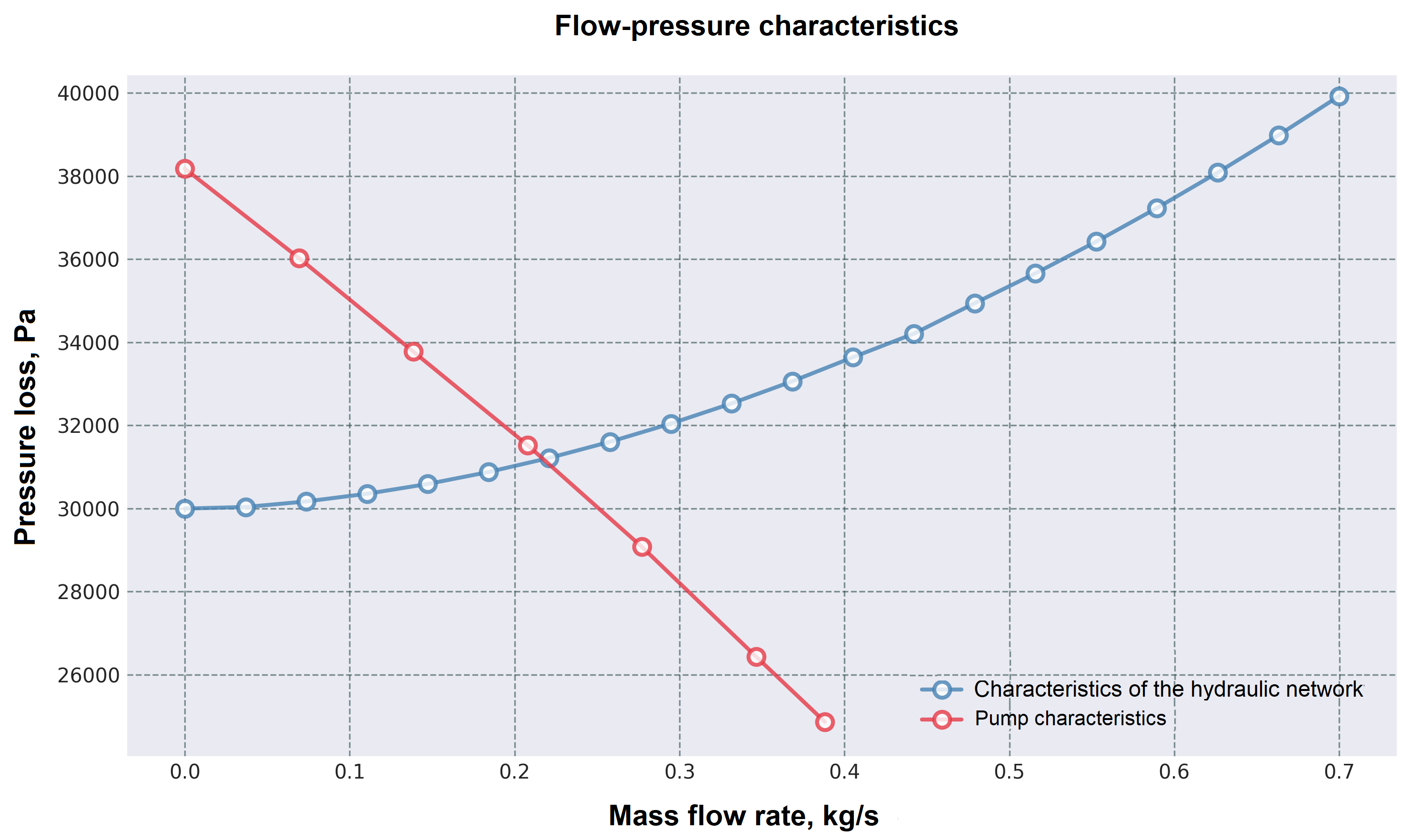
Fig. 2. Pump and network characteristics graphs#
3. Sequential operation of pumps on the network#
3.1. Description#
Sequential operation of pumps in a network is used in cases where the pressure developed by one pump is insufficient to supply liquid to a given height, or in cases where sequential connection of pumps allows for the supply of the required flow rate with a given network characteristic. [1]
With this connection scheme, the discharge pipe of one pump is connected to the suction pipe of the second pump.
3.2. Construction of characteristics#
The summary performance characteristic of two pumps connected in series is constructed by adding their ordinates at the same flow rates, since the pressure developed by the pumps operating in series is equal to the sum of the pressures developed by each of these pumps. [1]
Let’s construct the characteristics of two identical Wilo Star-RS 25/4 pumps operating sequentially using JupyterLite.
Code for building characteristics
# Импорт необходимых библиотек
import piplite
import pandas as pd

# Характеристика сети
system_head_curve_df = pd.DataFrame({
    'massFlowRate': [0.000000, 0.036842, 0.073684, 0.110526, 0.147368, 0.184211,
                     0.221053, 0.257895, 0.294737, 0.331579, 0.368421, 0.405263,
                     0.442105, 0.478947, 0.515789, 0.552632, 0.589474, 0.626316,
                     0.663158, 0.700000],
    'pressureDrop': [30000.000000, 30037.216415, 30171.196080, 30356.192800,
                     30591.674870, 30879.679700, 31218.609300, 31607.275800,
                     32044.753000, 32530.294700, 33063.283000, 33643.198700,
                     34209.597000, 34942.093300, 35660.350000, 36424.071000,
                     37232.990700, 38086.874000, 38985.507000, 39928.697000]
})
# Характеристика насоса Wilo Star-RS 25/4
pump_curve_df = pd.DataFrame({
    'massFlowRate': [0.0, 0.0693, 0.1386, 0.2079, 0.2772, 0.3465, 0.3881],
    'pressureDrop': [38182.5, 36028.6, 33776.8, 31525.0, 29077.4, 26434.0, 24867.6]
})

# Получаем характеристику двух последовательно работающих насосов
pump_series_curve_df = pd.DataFrame({
    'massFlowRate': [0.0, 0.0693, 0.1386, 0.2079, 0.2772, 0.3465, 0.3881],
    'pressureDrop': [38182.5, 36028.6, 33776.8, 31525.0, 29077.4, 26434.0, 24867.6]
})
pump_series_curve_df['pressureDrop'] = pump_series_curve_df['pressureDrop'] * 2

# Импортируем и устанавливаем необходимые библиотеки для визуализации
import matplotlib.pyplot as plt
await piplite.install("seaborn")
import seaborn as sns

def plot_pressure_drop_curve(system_head_curve_df, pump_curve__df, pump_series_curve_df, figsize=(10, 6)):
    """
    Создает график зависимости потерь давления от массового расхода.

    Parameters:
    -----------
    system_head_curve_df : pd.DataFrame
        DataFrame с колонками 'massFlowRate' и 'pressureDrop' для характеристики сети
    pump_curve__df : pd.DataFrame
        DataFrame с колонками 'massFlowRate' и 'pressureDrop' для характеристики насоса
    pump_series_curve_df: pd.DataFrame
        DataFrame с колонками 'massFlowRate' и 'pressureDrop' для характеристики двух последовательно работающих насосов
    figsize : tuple
        Размер графика в дюймах (ширина, высота)
    """

    # Настройка стиля графика
    plt.style.use('seaborn-v0_8-dark')

    # Создаем фигуру и оси с указанным размером
    fig, ax = plt.subplots(figsize=figsize, dpi=100)

    # Фильтруем данные, исключая NaN значения для чистоты графика
    clean_data = system_head_curve_df.dropna(subset=['pressureDrop'])
    # Данные для насоса
    clean_pump_data = pump_curve__df.dropna(subset=['pressureDrop'])
    # Данные для двух последовательных насосов
    clean_pump_series_data = pump_series_curve_df.dropna(subset=['pressureDrop'])
    # Проверяем, есть ли данные для отображения
    if len(clean_data) == 0:
        print("Нет данных для построения графика (все значения NaN)")
        return

    # Создаем основной график - линию с маркерами
    # Используем маркеры 'o' для точек и линию для соединения

    # График РНХ сети
    ax.plot(clean_data['massFlowRate'],
            clean_data['pressureDrop'],
            marker='o',                # Маркеры в виде кружков
            markersize=8,              # Размер маркеров
            linewidth=2,               # Толщина линии
            color='steelblue',         # Цвет линии
            alpha=0.8,                 # Прозрачность
            label='Характеристика гидравлической сети',   # Метка для легенды
            markerfacecolor='white',   # Заливка маркеров
            markeredgewidth=2)         # Толщина обводки маркеров

    # График РНХ насоса
    ax.plot(clean_pump_data['massFlowRate'],
            clean_pump_data['pressureDrop'],
            marker='o',                # Маркеры в виде кружков
            markersize=8,              # Размер маркеров
            linewidth=2,               # Толщина линии
            color='#e63946',            # Цвет линии
            alpha=0.8,                 # Прозрачность
            label='Характеристика насоса',   # Метка для легенды
            markerfacecolor='white',   # Заливка маркеров
            markeredgewidth=2)         # Толщина обводки маркеров

    # График РНХ последовательно работающих насосов
    ax.plot(clean_pump_series_data['massFlowRate'],
            clean_pump_series_data['pressureDrop'],
            marker='o',                # Маркеры в виде кружков
            markersize=8,              # Размер маркеров
            linewidth=2,               # Толщина линии
            color='#ffd166',            # Цвет линии
            alpha=0.8,                 # Прозрачность
            label='Характеристика двух последовательно работающих насосов',   # Метка для легенды
            markerfacecolor='white',   # Заливка маркеров
            markeredgewidth=2)         # Толщина обводки маркеров

    # Настройка осей графика
    ax.set_xlabel('Массовый расход, кг/с',
                  fontsize=12,
                  fontweight='bold',
                  labelpad=10)  # Отступ подписи от оси

    ax.set_ylabel('Потери давления, Па',
                  fontsize=12,
                  fontweight='bold',
                  labelpad=10)  # Отступ подписи от оси

    # Заголовок графика
    ax.set_title('Расходно-напорная характеристика',
                 fontsize=14,
                 fontweight='bold',
                 pad=20)  # Отступ заголовка

    # Добавляем сетку
    ax.grid(True, which='both', linestyle='--', color='#2F4F4F', alpha=0.6)

    # Настраиваем пределы осей с небольшим запасом
    x_min, x_max = clean_data['massFlowRate'].min(), clean_data['massFlowRate'].max()
    y_min, y_max = clean_data['pressureDrop'].min(), clean_pump_series_data['pressureDrop'].max()

    # Добавляем 5% запаса по осям
    x_padding = (x_max - x_min) * 0.05
    y_padding = (y_max - y_min) * 0.05

    ax.set_xlim(x_min - x_padding, x_max + x_padding)
    ax.set_ylim(y_min - 12 * y_padding, y_max + y_padding)

    # Добавляем легенду с настройками позиционирования
    ax.legend(loc='lower right',
          bbox_to_anchor=(1.0, 0.012),
          fontsize=10,
          framealpha=0.9,
          facecolor='#2F4F4F',
          edgecolor='white')

    # Настраиваем внешний вид графика
    # Убираем лишние отступы
    plt.tight_layout()
    # Отображаем график
    plt.show()
    # Возвращаем объекты фигуры и осей для возможной дальнейшей настройки
    return fig, ax

# Создаем график
fig, ax = plot_pressure_drop_curve(system_head_curve_df, pump_curve_df,pump_series_curve_df)
After executing the code, we obtain the following characteristics, Fig. 3:
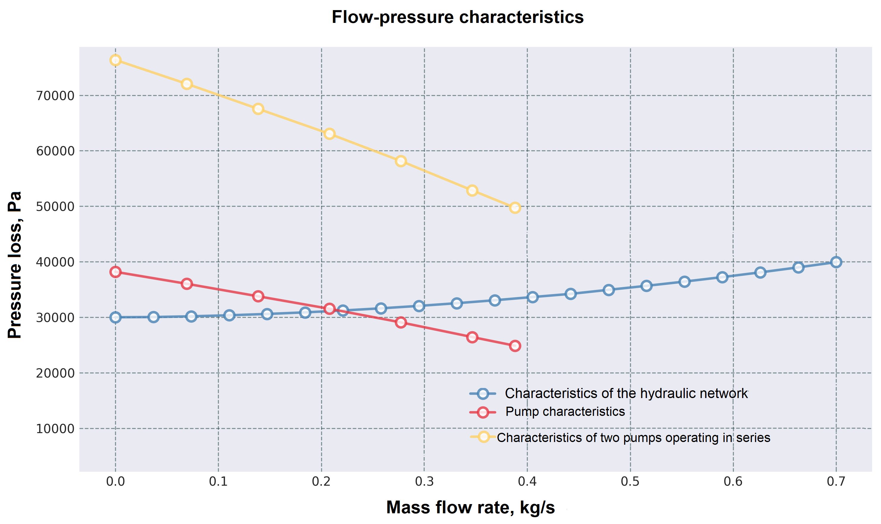
Fig. 3 Pump sequential operation curve#
To determine the operating point, the points of the graph of the joint operation of the pumps are not enough, we will add points based on the data on the FPC of the pump and repeat the construction (see Fig. 4 below).
Required data changes
# Характеристика насоса Wilo Star-RS 25/4
pump_curve_df = pd.DataFrame({
    'massFlowRate': [0.0, 0.0693, 0.1386, 0.2079, 0.2772, 0.3465, 0.3881, 0.4851, 0.5544, 0.6238],
    'pressureDrop': [38182.5, 36028.6, 33776.8, 31525.0, 29077.4, 26434.0, 24867.6, 21049.3, 18112.2, 15175.1]
})

# Получаем характеристику двух последовательно работающих насосов
pump_series_curve_df = pd.DataFrame({
    'massFlowRate': [0.0, 0.0693, 0.1386, 0.2079, 0.2772, 0.3465, 0.3881, 0.4851, 0.5544, 0.6238],
    'pressureDrop': [38182.5, 36028.6, 33776.8, 31525.0, 29077.4, 26434.0, 24867.6, 21049.3, 18112.2, 15175.1]
})
pump_series_curve_df['pressureDrop'] = pump_series_curve_df['pressureDrop'] * 2
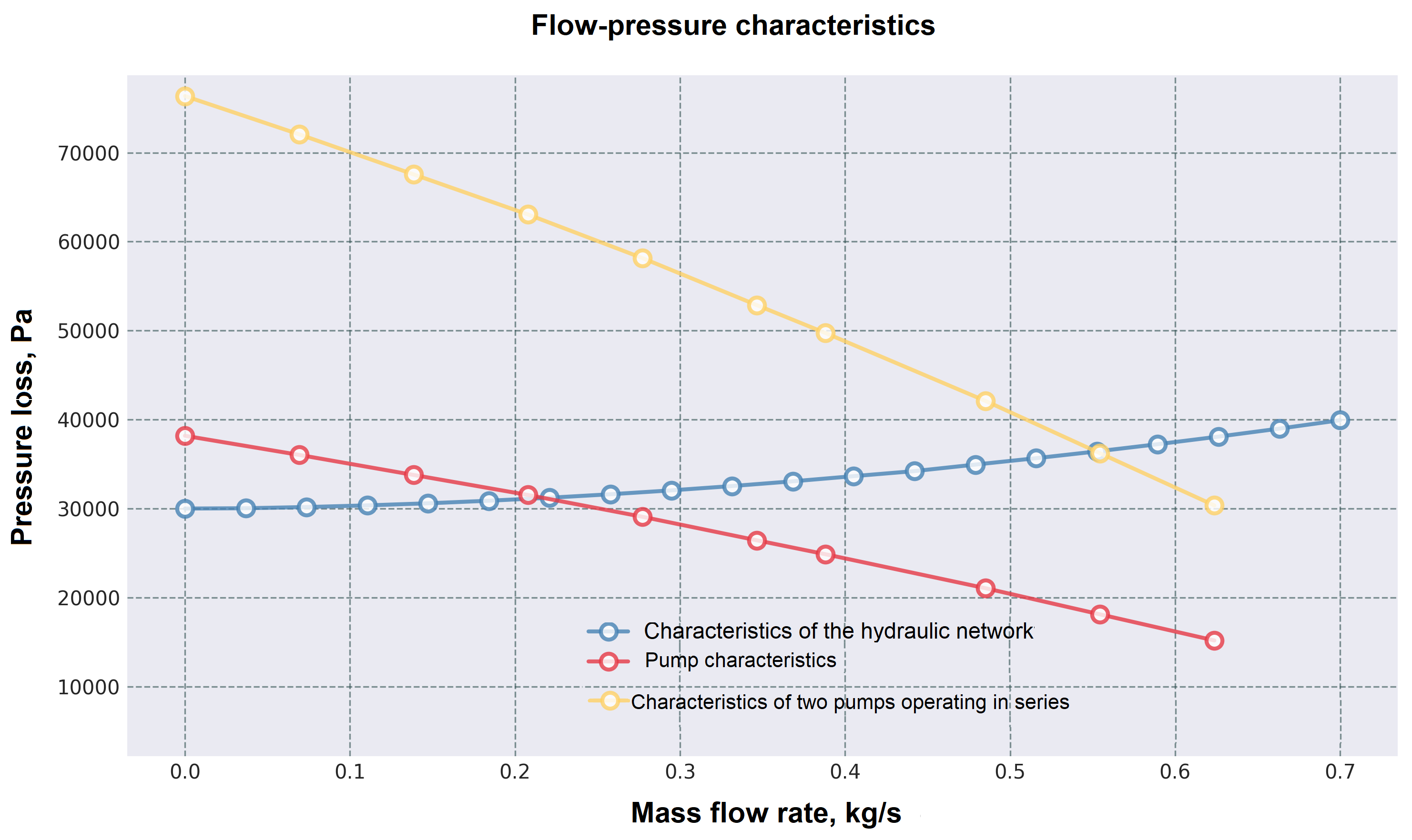
Fig. 4 Curve of sequential operation of pumps with a large number of design points#
Thus, the operating point of the pump corresponds to a flow rate of about 0.56 [kg/s].
Let’s move on to the model and calculate the operating point in it.
3.3. Implementation of sequential operation of pumps in a mathematical model#
Add another pump after the first one, as shown in Fig. 5:
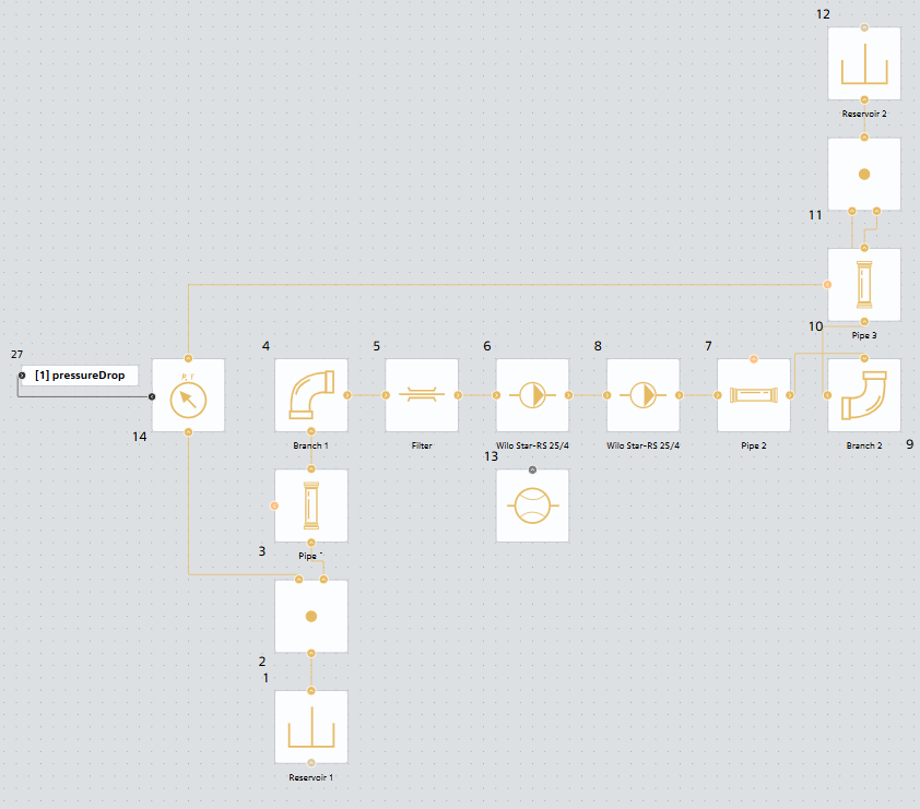
Fig. 5 Model of sequential operation of pumps#
Run the model and determine the operating point using the flow sensor, Fig. 6:
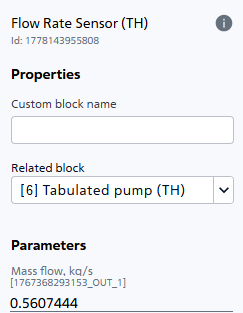
Fig. 6 Flow rate of the medium during sequential operation of two Wilo Star-RS 25/4 pumps#
The flow rate value is 0.5607444 [kg/s], which corresponds to the previously constructed curves and the graphically determined operating point.
4. Parallel operation of pumps on the network#
4.1. Description#
Parallel operation of pumps is used in the following cases:
To increase the overall system performance (feed)
To ensure redundancy and improve system reliability
For flexible performance control and energy savings
With this connection scheme, the discharge pipe of each pump is connected to the general system.
4.2. Construction of characteristics#
The summary performance characteristic of two parallel-connected pumps is constructed by adding their abscissas at the same pressures.
The total flow rate of pumps operating in parallel in a common system is less than the sum of the flows of the same pumps when they operate separately.
Hint
As the total flow rate of the medium supplied to the system increases, pressure losses increase, and consequently the pressure required to supply a given flow rate also increases, which entails a decrease in the flow rate of each pump. [1]
Let’s construct the characteristics of two identical Wilo Star-RS 25/4 pumps operating in parallel using JupyterLite.
Code for building characteristics
# Импорт необходимых библиотек
import piplite
import pandas as pd

# Характеристика сети
system_head_curve_df = pd.DataFrame({
    'massFlowRate': [0.000000, 0.036842, 0.073684, 0.110526, 0.147368, 0.184211,
                     0.221053, 0.257895, 0.294737, 0.331579, 0.368421, 0.405263,
                     0.442105, 0.478947, 0.515789, 0.552632, 0.589474, 0.626316,
                     0.663158, 0.700000],
    'pressureDrop': [30000.000000, 30037.216415, 30171.196080, 30356.192800,
                     30591.674870, 30879.679700, 31218.609300, 31607.275800,
                     32044.753000, 32530.294700, 33063.283000, 33643.198700,
                     34209.597000, 34942.093300, 35660.350000, 36424.071000,
                     37232.990700, 38086.874000, 38985.507000, 39928.697000]
})

# Характеристика насоса Wilo Star-RS 25/4
pump_curve_df = pd.DataFrame({
    'massFlowRate': [0.0, 0.0693, 0.1386, 0.2079, 0.2772, 0.3465, 0.3881],
    'pressureDrop': [38182.5, 36028.6, 33776.8, 31525.0, 29077.4, 26434.0, 24867.6]
})

# Получаем характеристику двух параллельно работающих насосов
pump_parallel_curve_df = pd.DataFrame({
    'massFlowRate': [0.0, 0.0693, 0.1386, 0.2079, 0.2772, 0.3465, 0.3881],
    'pressureDrop': [38182.5, 36028.6, 33776.8, 31525.0, 29077.4, 26434.0, 24867.6]
})
pump_parallel_curve_df['massFlowRate'] = pump_parallel_curve_df['massFlowRate'] * 2


# Импортируем и устанавливаем необходимые библиотеки для визуализации
import matplotlib.pyplot as plt
await piplite.install("seaborn")
import seaborn as sns

def plot_pressure_drop_curve(system_head_curve_df, pump_curve__df, pump_parallel_curve_df, figsize=(10, 6)):
    """
    Создает график зависимости потерь давления от массового расхода.

    Parameters:
    -----------
    system_head_curve_df : pd.DataFrame
        DataFrame с колонками 'massFlowRate' и 'pressureDrop' для характеристики сети
    pump_curve__df : pd.DataFrame
        DataFrame с колонками 'massFlowRate' и 'pressureDrop' для характеристики насоса
    pump_parallel_curve_df: pd.DataFrame
        DataFrame с колонками 'massFlowRate' и 'pressureDrop' для характеристики двух параллельно работающих насосов
    figsize : tuple
        Размер графика в дюймах (ширина, высота)
    """

    # Настройка стиля графика
    plt.style.use('seaborn-v0_8-dark')

    # Создаем фигуру и оси с указанным размером
    fig, ax = plt.subplots(figsize=figsize, dpi=100)

    # Фильтруем данные, исключая NaN значения для чистоты графика
    clean_data = system_head_curve_df.dropna(subset=['pressureDrop'])
    # Данные для насоса
    clean_pump_data = pump_curve__df.dropna(subset=['pressureDrop'])
    # Данные для двух параллельно работающих насосов
    clean_pump_parallel_data = pump_parallel_curve_df.dropna(subset=['pressureDrop'])
    # Проверяем, есть ли данные для отображения
    if len(clean_data) == 0:
        print("Нет данных для построения графика (все значения NaN)")
        return

    # Создаем основной график - линию с маркерами
    # Используем маркеры 'o' для точек и линию для соединения

    # График РНХ сети
    ax.plot(clean_data['massFlowRate'],
            clean_data['pressureDrop'],
            marker='o',                # Маркеры в виде кружков
            markersize=8,              # Размер маркеров
            linewidth=2,               # Толщина линии
            color='steelblue',         # Цвет линии
            alpha=0.8,                 # Прозрачность
            label='Характеристика гидравлической сети',   # Метка для легенды
            markerfacecolor='white',   # Заливка маркеров
            markeredgewidth=2)         # Толщина обводки маркеров

    # График РНХ насоса
    ax.plot(clean_pump_data['massFlowRate'],
            clean_pump_data['pressureDrop'],
            marker='o',                # Маркеры в виде кружков
            markersize=8,              # Размер маркеров
            linewidth=2,               # Толщина линии
            color='#e63946',            # Цвет линии
            alpha=0.8,                 # Прозрачность
            label='Характеристика насоса',   # Метка для легенды
            markerfacecolor='white',   # Заливка маркеров
            markeredgewidth=2)         # Толщина обводки маркеров

    # График РНХ параллельно работающих насосов
    ax.plot(clean_pump_parallel_data['massFlowRate'],
            clean_pump_parallel_data['pressureDrop'],
            marker='o',                # Маркеры в виде кружков
            markersize=8,              # Размер маркеров
            linewidth=2,               # Толщина линии
            color='#ffd166',            # Цвет линии
            alpha=0.8,                 # Прозрачность
            label='Характеристика двух параллельно работающих насосов',   # Метка для легенды
            markerfacecolor='white',   # Заливка маркеров
            markeredgewidth=2)         # Толщина обводки маркеров

    # Настройка осей графика
    ax.set_xlabel('Массовый расход, кг/с',
                  fontsize=12,
                  fontweight='bold',
                  labelpad=10)  # Отступ подписи от оси

    ax.set_ylabel('Потери давления, Па',
                  fontsize=12,
                  fontweight='bold',
                  labelpad=10)  # Отступ подписи от оси

    # Заголовок графика
    ax.set_title('Расходно-напорная характеристика',
                 fontsize=14,
                 fontweight='bold',
                 pad=20)  # Отступ заголовка

    # Добавляем сетку
    ax.grid(True, which='both', linestyle='--', color='#2F4F4F', alpha=0.6)

    # Настраиваем пределы осей с небольшим запасом
    x_min, x_max = clean_data['massFlowRate'].min(), clean_pump_parallel_data['massFlowRate'].max()
    y_min, y_max = clean_pump_parallel_data['pressureDrop'].min(), clean_data['pressureDrop'].max()

    # Добавляем 5% запаса по осям
    x_padding = (x_max - x_min) * 0.05
    y_padding = (y_max - y_min) * 0.05

    ax.set_xlim(x_min - x_padding, x_max + x_padding)
    ax.set_ylim(y_min - 12 * y_padding, y_max + y_padding)

    # Добавляем легенду с настройками позиционирования
    ax.legend(loc='lower right',
          bbox_to_anchor=(1.0, 0.012),
          fontsize=10,
          framealpha=0.9,
          facecolor='#2F4F4F',
          edgecolor='white')

    # Настраиваем внешний вид графика
    # Убираем лишние отступы
    plt.tight_layout()
    # Отображаем график
    plt.show()
    # Возвращаем объекты фигуры и осей для возможной дальнейшей настройки
    return fig, ax

# Создаем график
fig, ax = plot_pressure_drop_curve(system_head_curve_df, pump_curve_df,pump_parallel_curve_df)
After executing the code, we obtain the following characteristics, Fig. 7:
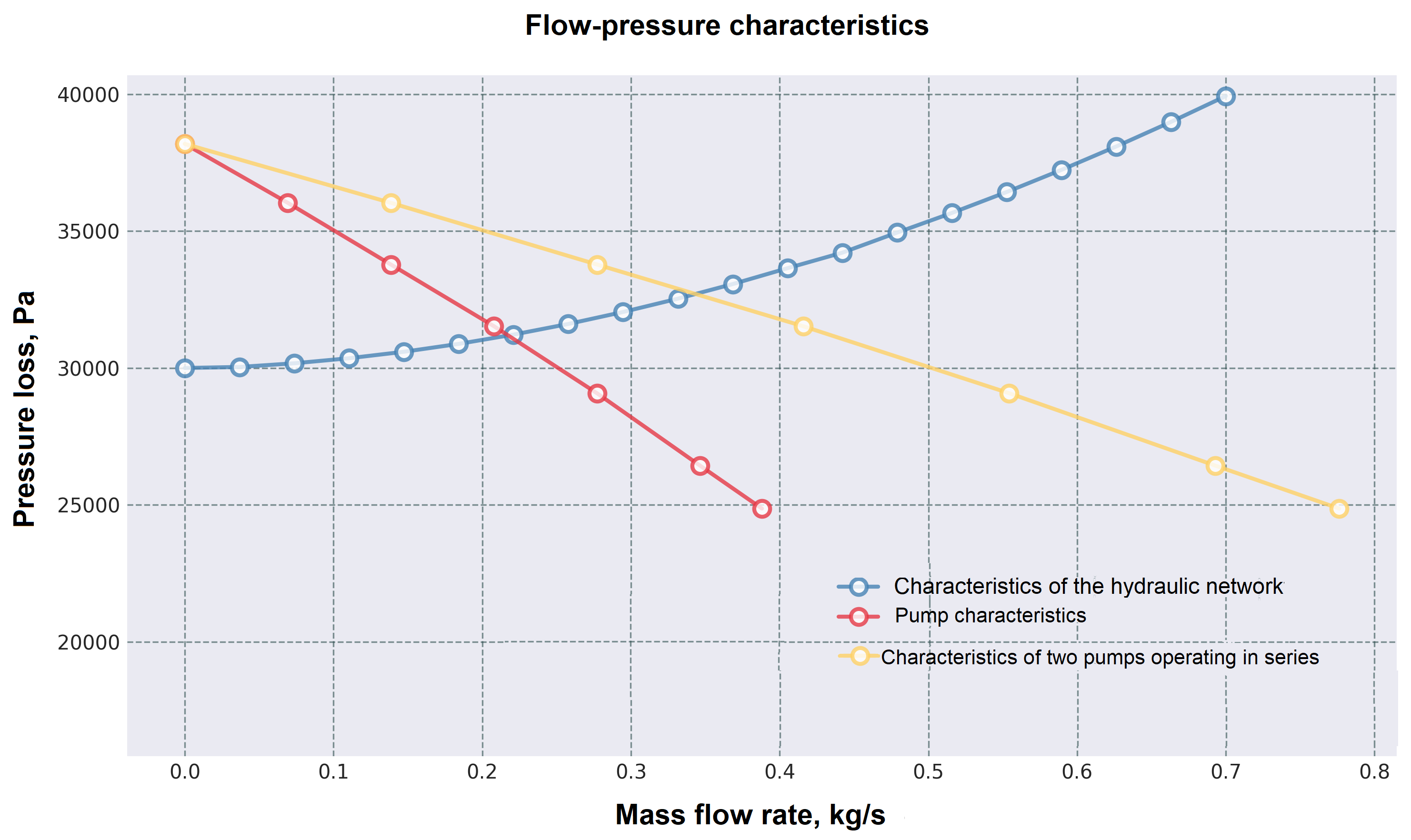
Fig. 7 Parallel operation curve of pumps#
Thus, the operating point of the pump corresponds to a flow rate of about 0.35 [kg/s].
Let’s move on to the model and calculate the operating point in it.
4.3. Implementation of parallel operation of pumps in a mathematical model#
Copy the model used to study the series operation of pumps, arrange and connect the pumps in parallel as shown in Fig. 8. Specify Pipe 2 as the linked block for the flow sensor to measure the total flow in the network, rather than the flow of a single pump.
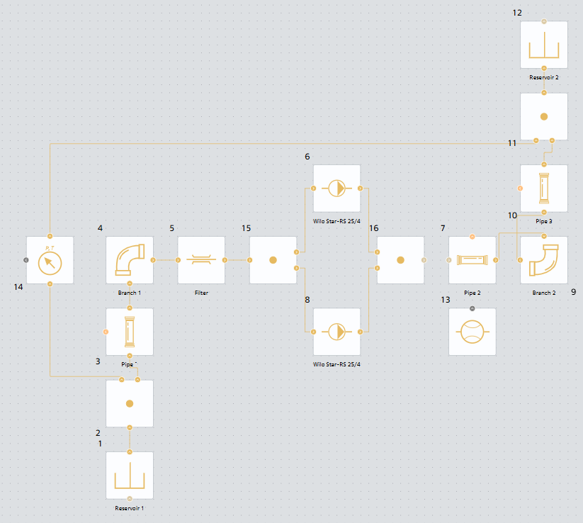
Fig. 8 Model of parallel operation of pumps#
Run the model and determine the operating point using the flow sensor, Fig. 9:
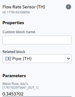
Fig. 9 Flow rate of the medium during parallel operation of two Wilo Star-RS 25/4 pumps#
The flow rate value is 0.3453702 [kg/s], which corresponds to the previously constructed curves and the graphically determined operating point.
5. Conclusions#
During the course of the tutorial, the methodology of comparative analysis of two basic schemes of joint operation of pumps - sequential and parallel - using SW REPEAT VISION was successfully mastered. The practical work allowed us to implement a full cycle of engineering research: from constructing theoretical summary characteristics based on classical methods (summing ordinates for a series connection and abscissas for a parallel connection) to verifying these calculations using mathematical models.
System modeling significantly simplifies the process of calculating the operation of a hydraulic system with pumping equipment and optimizes the process of setting up and selecting the necessary parameters (geometry, materials, configuration, equipment composition), reducing the pre-design stages of design. Ultimately, the reliability and energy efficiency of the final solution is increased.