Working with CSV files: exporting and importing simulation results

 When modeling, it is often necessary to save the calculation results for subsequent analysis in other programs (Excel, Python) or, conversely, to feed external data into the model - for example, real signals from sensors, tabular dependencies, previously obtained results of model calculations. For this purpose, REPEAT VISION provides the Export CSV and Import CSV blocks.

CSV (Comma-Separated Values) is a simple text format in which values ​​are separated by commas or semicolons, and the first row typically contains column headings.

 CSV files are often used for:

• data exchange between models;

• loading experimental measurements;

• preparation of test impacts;

• post-processing of results in Python, Excel.

 In this tutorial, we’ll build a model with two periodic signals (a sine wave and a square wave), export them to a CSV file, and then import that file back into the model, changing the interpolation and extrapolation settings. This will help us understand:

• how to set the amount of data to be written;

• how to control discretization;

• how do different types of interpolation and extrapolation affect import.

 Example of a graph imported using a CSV block, Fig. 1:

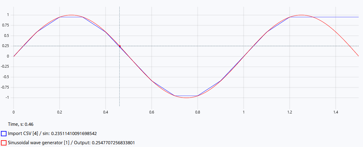
Fig. 1 Example of a graph imported using a CSV block

1.  Statement of the problem

 Create a model with two sources of periodic signals:

• sinusoidal: amplitude 1, frequency 1 [Hz];

• rectangular pulses: amplitude 1, frequency 1 [Hz], duty cycle 50%.

 Calculation time – 1.25 [s], integration step – 0.001 [s].

 These signals are fed to the Export CSV block, which saves them to a file with the specified headers and the selected discretization.

 Then the Import CSV block is installed, reading the previously acquired file. The import output should match the source. After this, the effects of various interpolation and extrapolation settings are demonstrated.

2.  Creating and setting up a project

 Create a new project, name it, for example, CSV_example.

 Set the following settings for the project (see Fig. 2 below):

1. Disable the Synchronization with real time option;

2. Set Simulation time to 1.25 [s];

3. Set Integration step to 1 [ms];

4. Set Sampling step to 1 [ms].

Important

In REPEAT VISION, decimal numbers are separated by a dot.

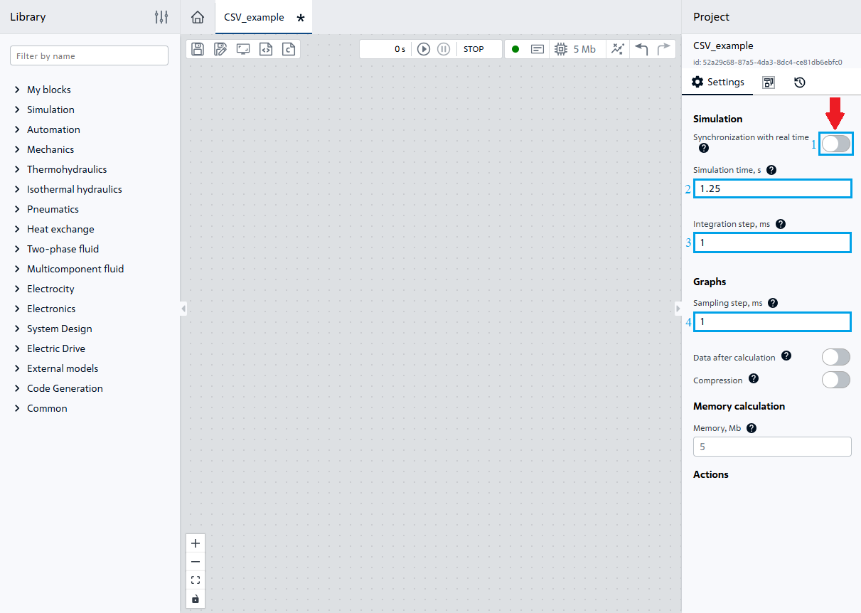
Fig. 2 Project setup

3.  Creating signal sources

 From the Automation section of the Suppliers add two generators and set the following property values ​​for them:

• Sinusoidal wave generator (see Fig. 3 below):

  • Amplitude - 1;

  • Vertical shift - 0.

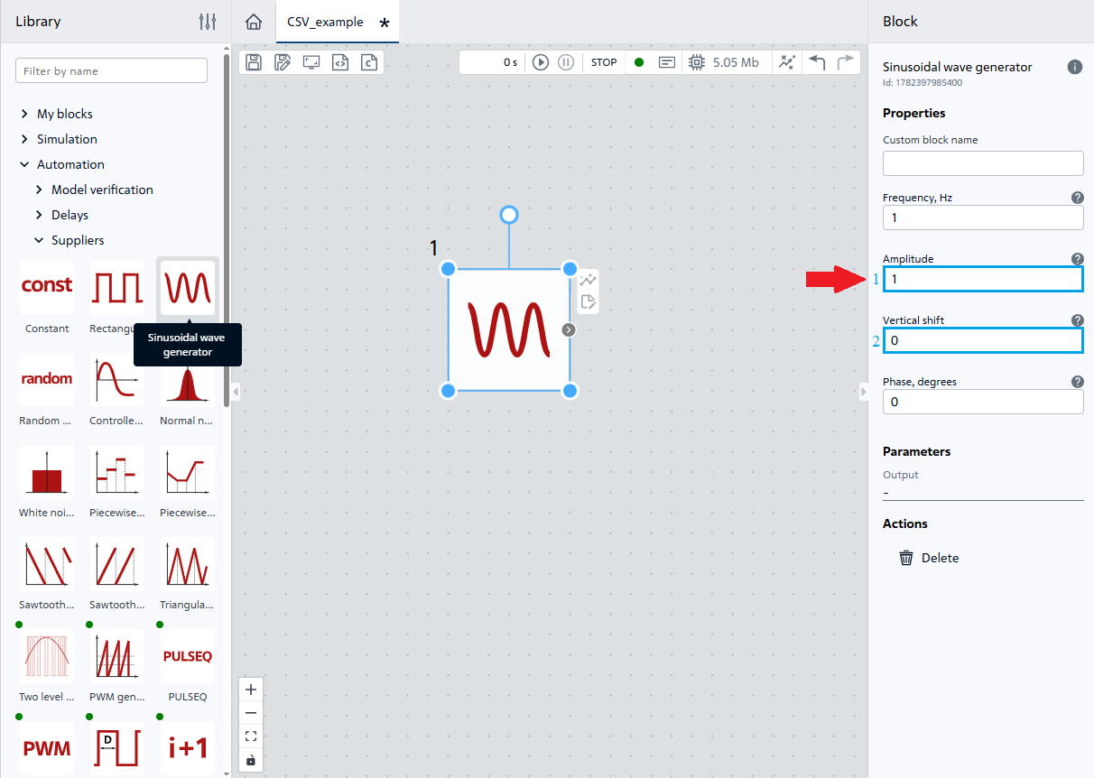
Fig. 3 Adding and configuring a sine wave generator

• Rectangular pulse generator (see Fig. 4 below):

  • Signal period a - 1000 [ms];

  • Signal duration b - 500 [ms];

  • Signal amplitude c - 1.

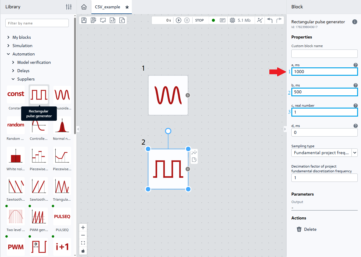
Fig. 4 Adding and configuring a pulse generator

4.  Graphing

 To plot signal source graphs using Visualization, and then run the model for a test calculation, it is necessary (see Fig. 5 and Fig. 6 below):

1. Open the Visualization tab, located on the bottom left panel;

2. Click LMB on the Add button;

3. In the drop-down list for plotting the first graph, select Sinusoidal wave generator [1];

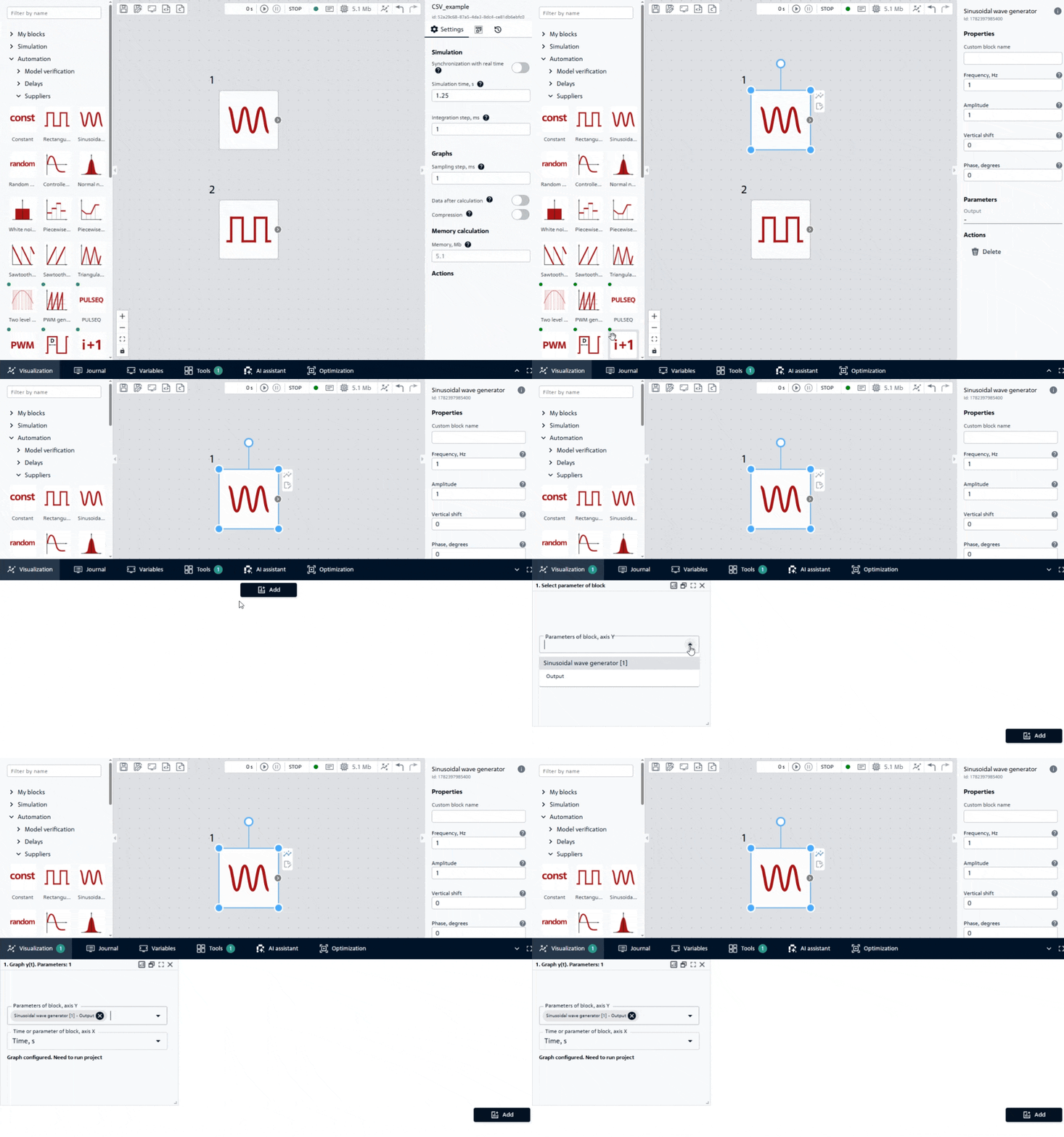
Fig. 5 Adding the first graph

4. LMB on the Add button located in the lower right corner;

5. In the drop-down list for plotting the second graph, select Rectangular pulse generator [2]

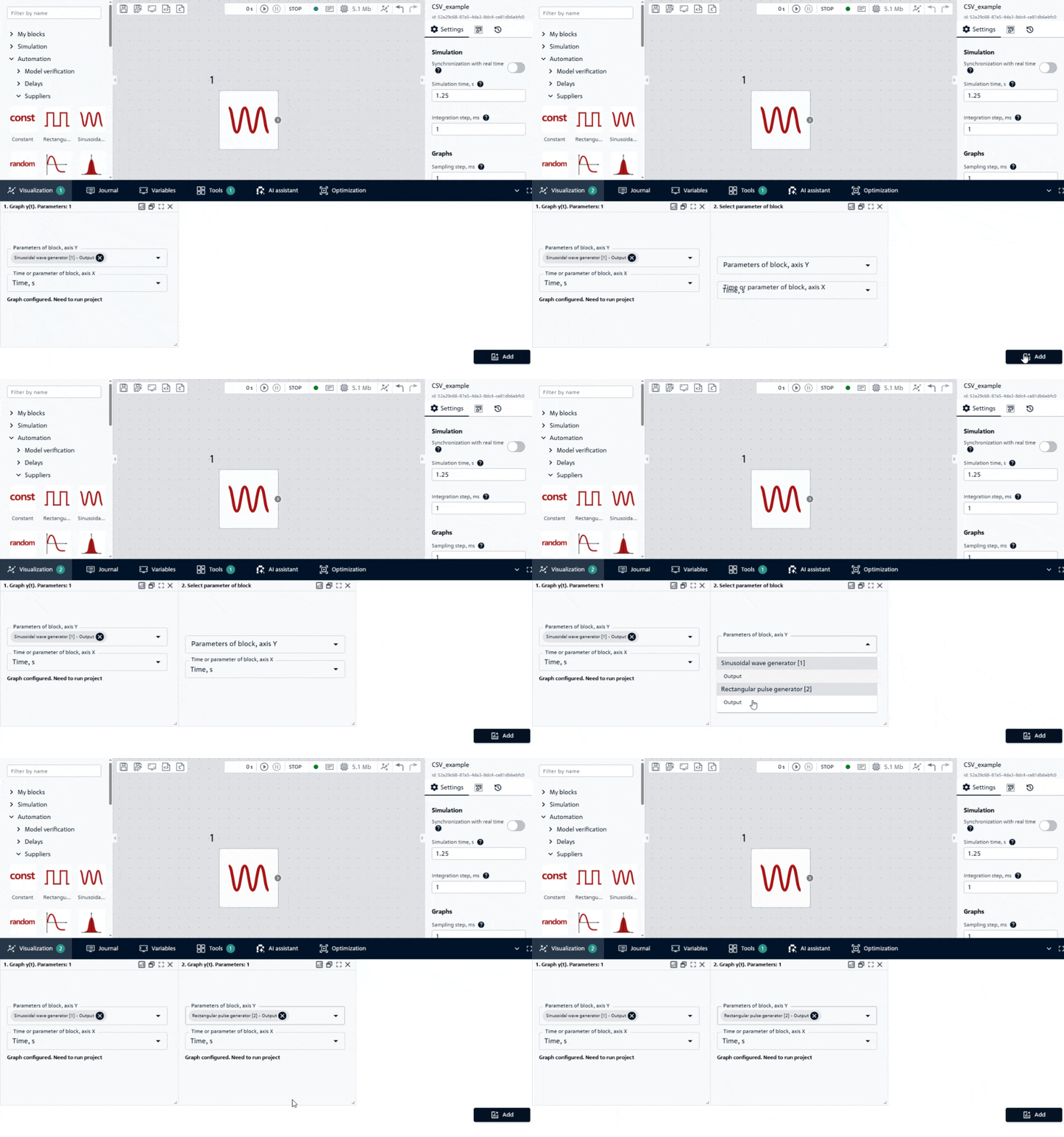
Fig. 6 Adding a second graph

 Then you need to run the calculation to obtain the following graphs, Fig. 7:

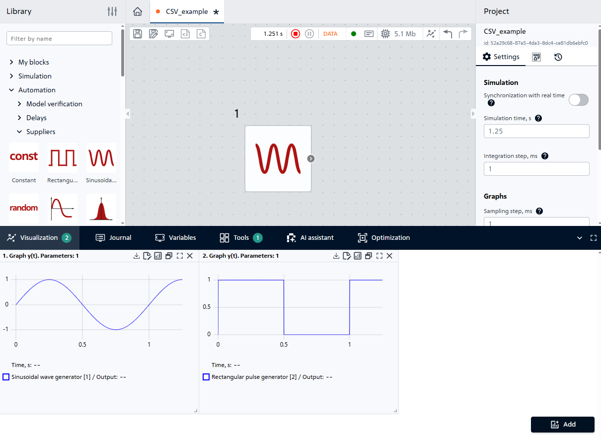
Fig. 7 Graphs of generated signals

 The model is ready to work with CSV blocks.

5.  Adding and connecting the “Export CSV” block

 From the External models section, add the Export CSV block (see Figure 8 below).

 Then we connect the Export CSV block according to Fig. 8:

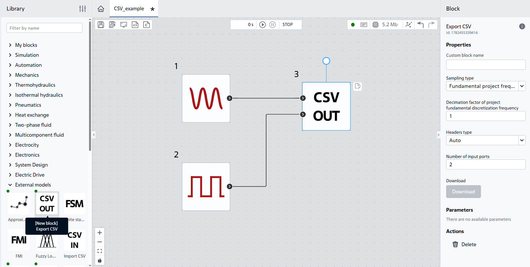
Fig. 8 Adding and connecting the Export CSV block

6.  Setting up the “Export CSV” block

6.1.  Setting up sampling

In the block properties, find Sampling type. There are three possible property options:

Type	Operating principle	Example
Fundamental project frequency decimation	Writes down every N-th point	If the calculation step = 0.001 [s], and the decimation N = 100, then a point will be included in the file every 0.1 [s]
Sample time	The recording occurs strictly at the specified time interval. This is the simplest and most straightforward method.	With a period of 0.05 [s], a point is recorded every 50 [ms]
Sampling frequency	It works like the period, but through the formula Period = 1 / Frequency	Frequency = 20 [Hz] → recording every 0.05 [s]

 Leave the default settings when Fundamental project frequency decimation is selected and Decimation factor of project fundamental discretization frequency = 1 is set (all points will be written to the .csv file).

6.2.  Customizing column headers

 The Headers type property has the following values:

• Auto - the block will create headings automatically;

• Custom - allows you to enter your own column names (separated by semicolons).

 Select the Custom value and in the Headers property enter the string: sin; square.

 As a result, the Export CSV block will be configured similarly to Fig. 9:

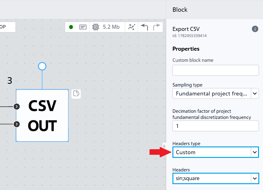
Fig. 9. Configuring the Export CSV block

7.  Starting the calculation and checking

 Run the model. After the calculation is complete, click the Download button in the Export CSV block. The .csv file will be generated and downloaded to your browser’s downloads folder, Fig. 10:

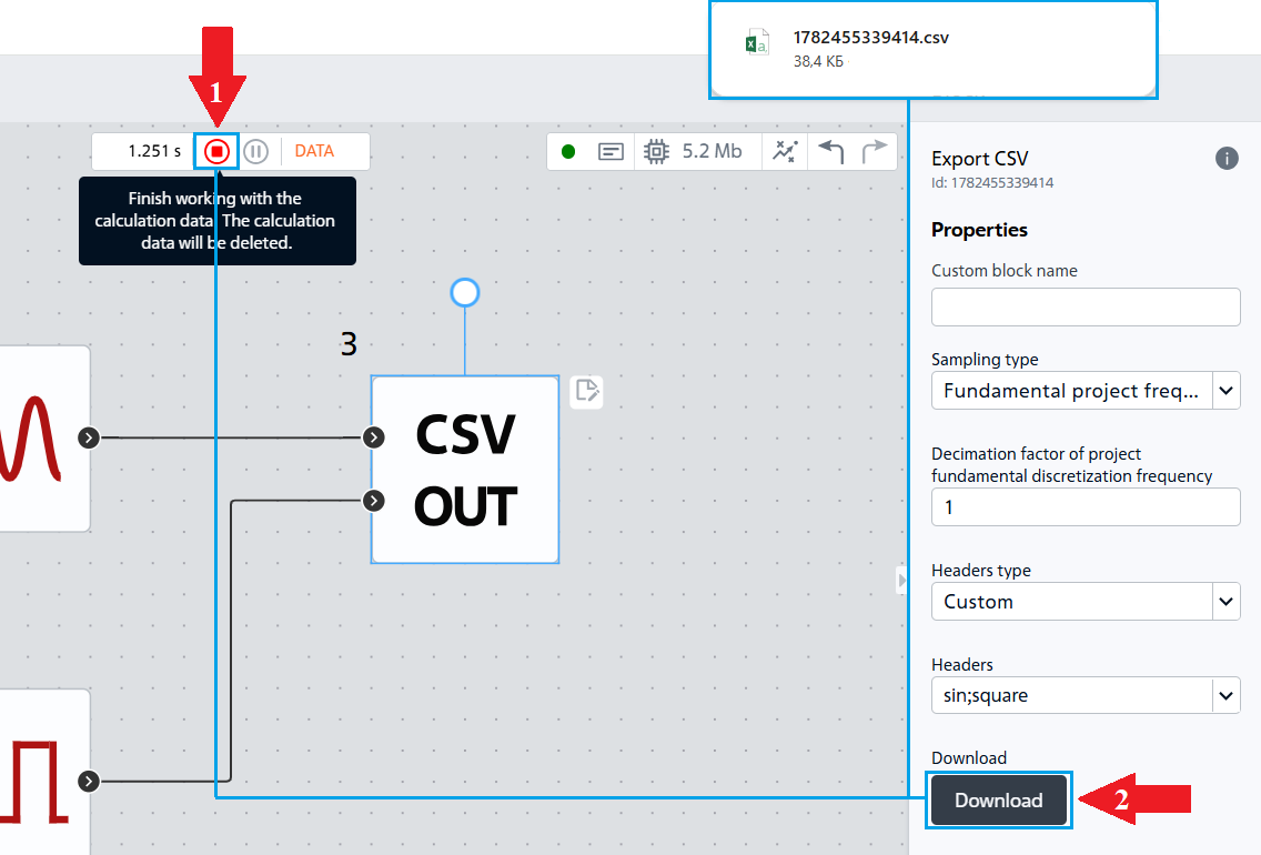
Fig. 10 Downloading calculation results

 When you open the downloaded .csv file, you should see three columns: t (time), sin (sine values), square (square wave values), Fig. 11:

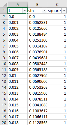
Fig. 11 The resulting .csv file

 For ease of reading the file name, we will rename the resulting CSV to resultsDecim1, Fig. 12:

Fig. 12 Renamed file

8.  The “Import CSV” block - reading and playing signals

 Now let’s load the saved data back into the model. To do this, add the Import CSV block from the External models library. The .csv file upload window will open automatically (see Fig. 13 below), into which you need to upload the last exported CSV.

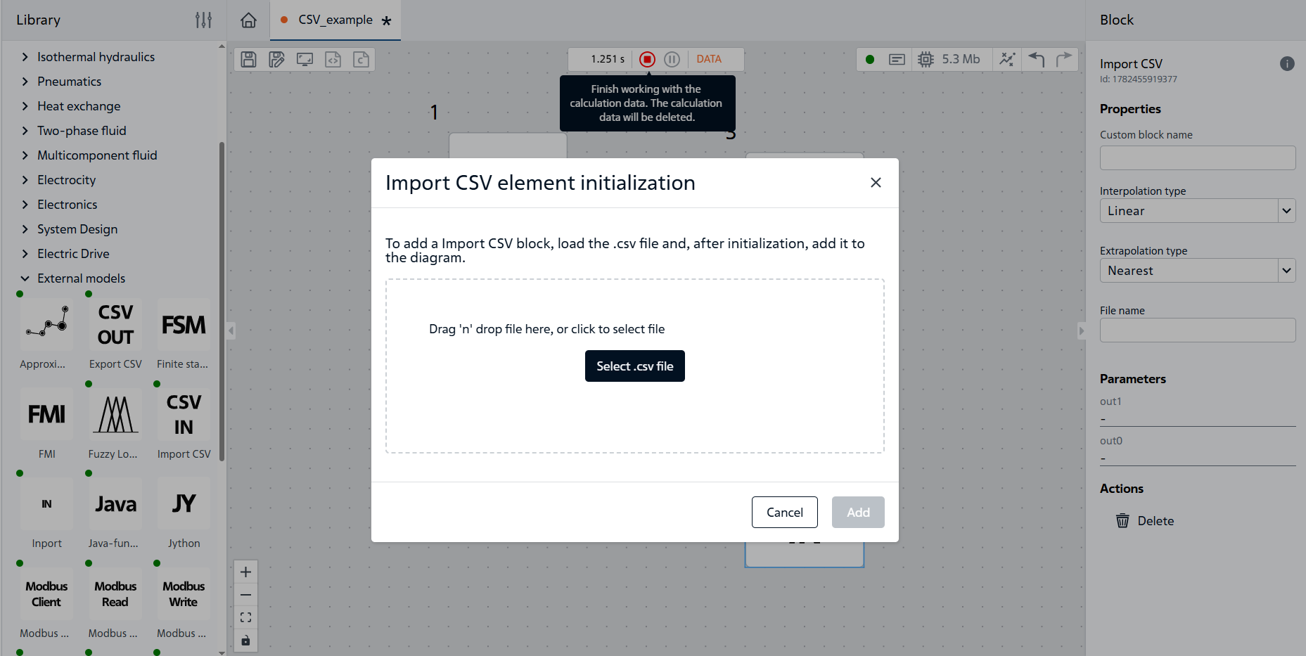
Fig. 13 File import

 After successful loading and initialization, click the Add button (see Fig. 14 below) so that the block appears on the canvas (see Fig. 15 below).

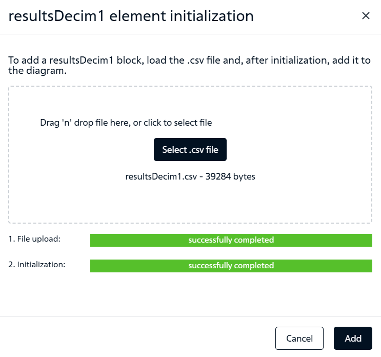
Fig. 14 Successful upload of .csv file

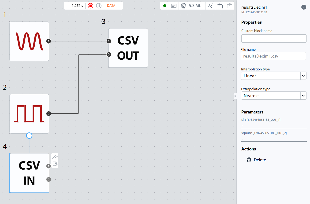
Fig. 15 Block added to the diagram

9.  Properties of the «Import CSV» block

9.1.  Setting up interpolation

The Interpolation type parameter determines how values ​​are reconstructed between points stored in the CSV:

• Linear - values ​​are connected by straight lines. This is the default. With a sufficiently small recording step, linear interpolation allows for highly accurate reconstruction of the original signal.

• Smooth (cubic spline interpolation) - constructs a smooth curve through all points.

Note

We leave the default value

9.2.  Setting up extrapolation

 The Extrapolation type parameter determines the output behavior when the simulation time goes beyond the time range specified in the CSV file (for example, the file contains data up to 1.25 [s], and the calculation goes up to 2 [s]):

• Nearest value - the output keeps the last value of the file;

• Linear - continues the line constructed from the last two points;

• Set to zero - outside the file the output becomes 0;

• No extrapolation - the block generates an error when calculating “further” than the last value of the file.

Note

We leave the default value

10.  Connection and launch

 Select the output signals of the Import CSV block to plot in the Visualization tab. Run the calculation.

 The graph (see Fig. 16 below) should exactly repeat the original signals: a sine wave and a rectangular pulse (if the export was with decimation 1 and the import with linear interpolation).

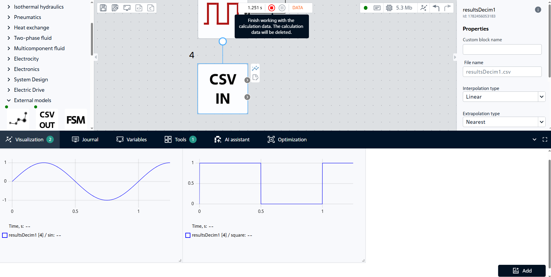
Fig. 16 Block signal values

 The imported signals are almost identical to the original ones, Fig. 17:

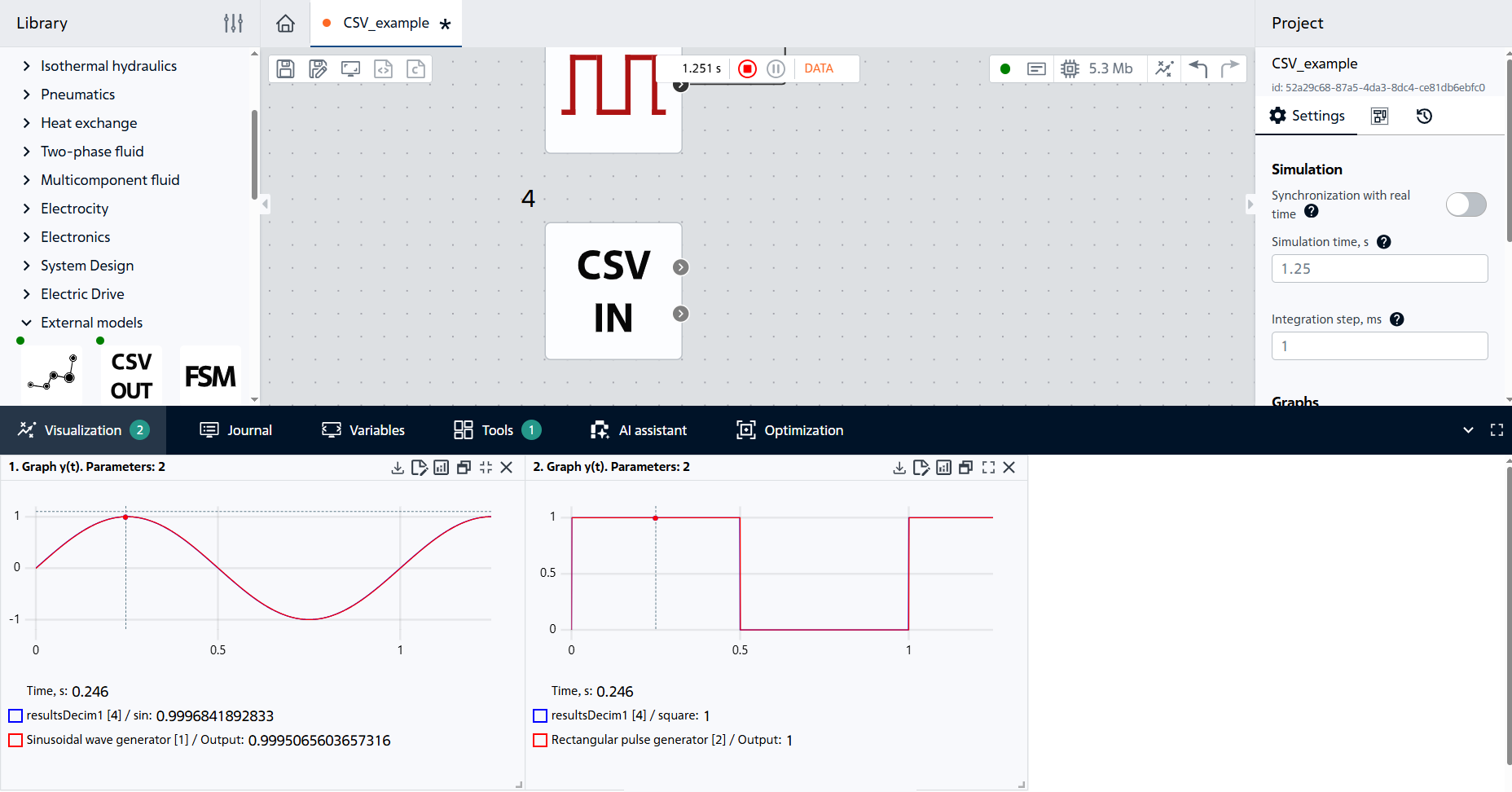
Fig. 17 Combined graphs

11.  Experimenting with settings

 We explore the configuration options for the Import CSV block based on the constructed sinusoidal signal.

11.1.  The impact of decimation on exports

 Let’s re-create the .csv file with a different decimation factor. In the CSV Export block, change the decimation factor to 100 (see Fig. 18 below), leaving the other properties at default. Run the calculation again (the sources must be connected).

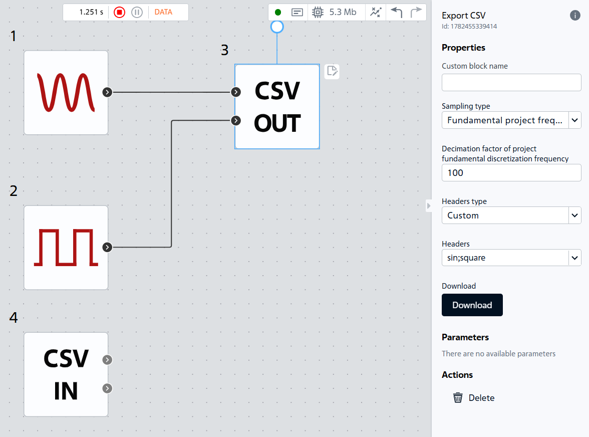
Fig. 18 Increasing the decimation coefficient

 Download and rename the CSV file to resultsDecim100, Fig. 19:

Fig. 19 Renamed file with increased coefficient

 Next, load the resulting .csv file into the project using the Import CSV block. Add a label for the Decimation = 100 block (see Figure 20 below). We won’t need the previous Import CSV block with Decimation = 1 for subsequent experiments.

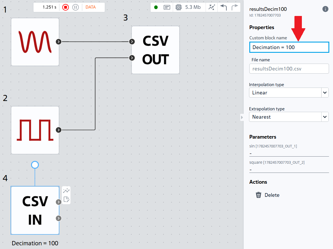
Fig. 20 Adding a block label

 Run the calculation and plot a graph combining the original sine wave and the imported .csv sine wave (see Fig. 21 below).

 You will see a broken line that only approximately follows the sine wave, particularly in the area of ​​the sine wave amplitude.

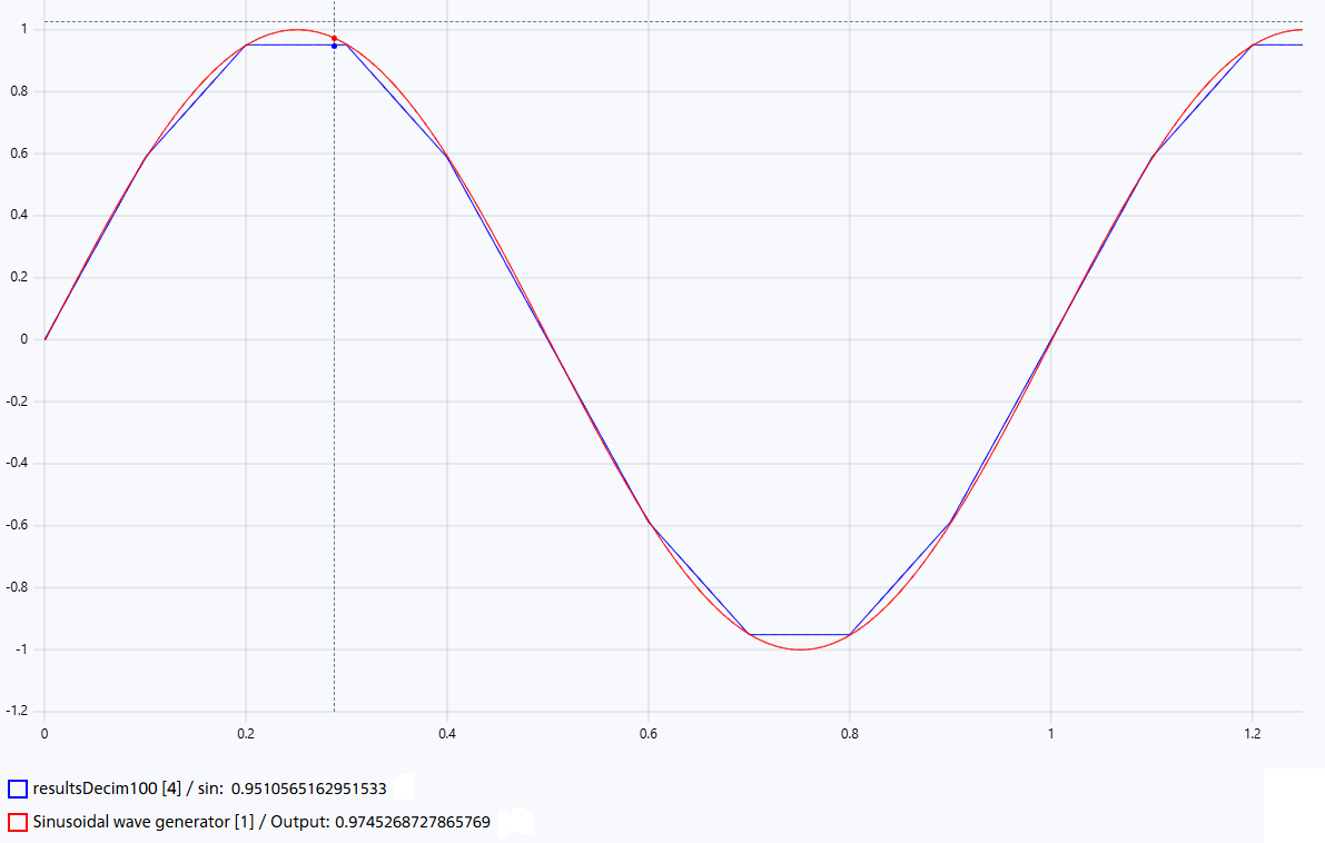
Fig. 21 Comparison of graphs

 Conclusion: Increasing the decimation coefficient reduces the number of stored points and decreases the size of the CSV file, but leads to a loss of signal reconstruction accuracy. For smooth signals this manifests itself as a broken graph shape, while for rapidly changing signals significant loss of information is possible.

11.2.  Comparison of interpolations

 In the same downloaded file, change the Interpolation type to Smooth (see Fig. 22 below). Run the calculation.

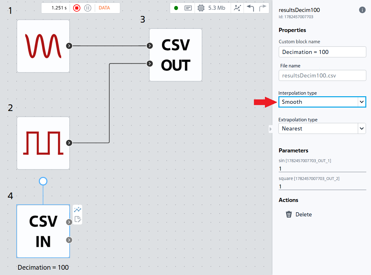
Fig. 22 Changing the interpolation type

 The sine wave becomes smoother, but the square wave begins to oscillate near the signal breaks, which distorts the signal front Fig. 23:

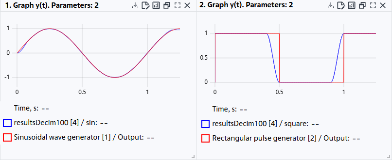
Fig. 23 Calculation results for the Smooth interpolation type

 Conclusion: Linear interpolation is better suited for signals with sharp changes and discontinuities, since it does not create additional oscillations between points. Smooth interpolation provides smoother recovery of smooth signals, but may cause spikes and wave-like distortions near sharp edges.

11.3.  Extrapolation

 Change the Simulation time from 1.25 to 2 [s]. Set the Interpolation type back to Linear. Then, successively select different Extrapolation type:

• Nearest value - after 1.25 [s] the output remains at the level of the last value (sine ≈ 1), Fig. 24:

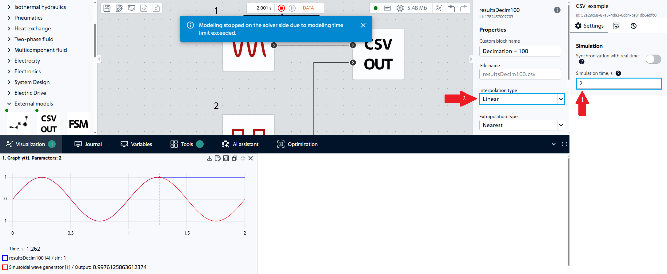
Fig. 24 Calculation results for the extrapolation type Nearest value

• Linear - the output continues to move along the straight line defined by the last two points, Fig. 25:

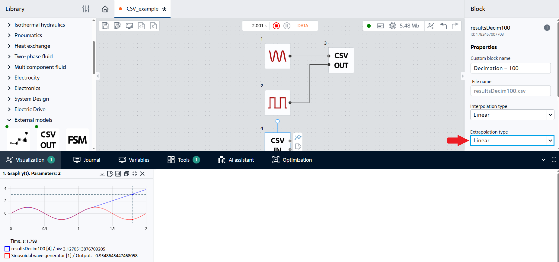
Fig. 25 Calculation results for the Linear extrapolation type

• Set to zero - after 1.25 [s] the output is reset, Fig. 26:

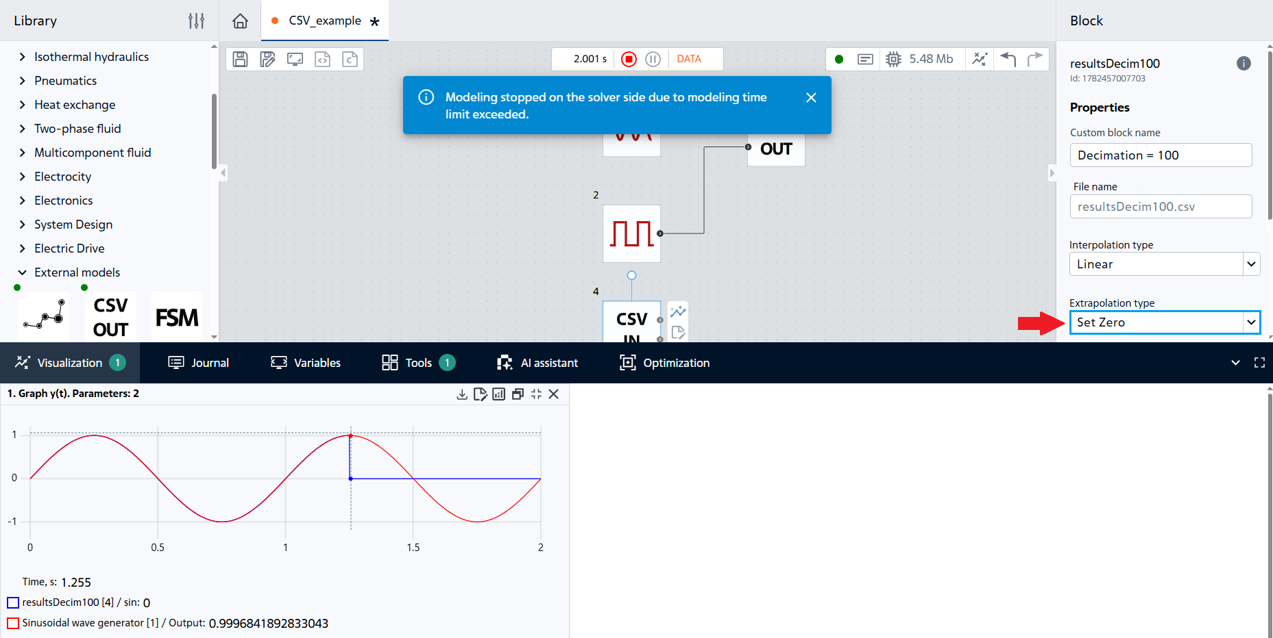
Fig. 26 Calculation results for the extrapolation type Set to zero

• No extrapolation – the calculation will fail because the block cannot calculate values ​​outside the data range, Fig. 27:

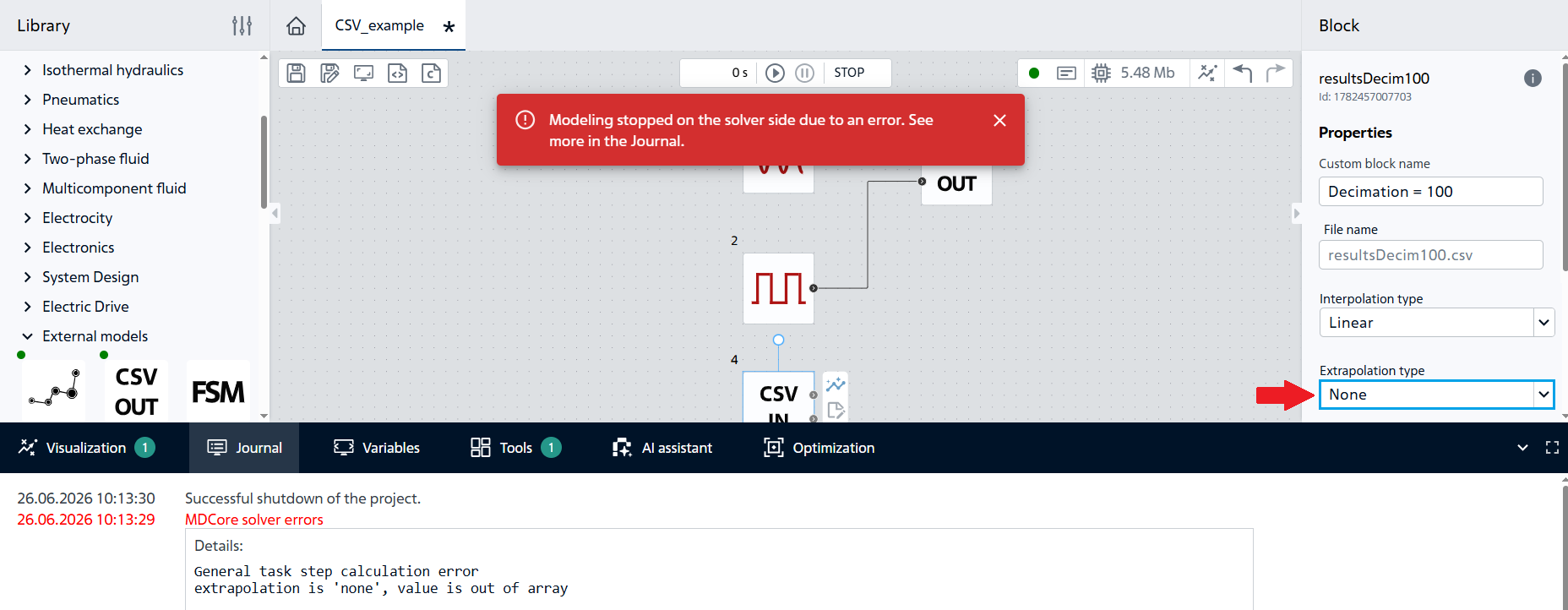
Fig. 27 Calculation results for the Without extrapolation type

 Output: The extrapolation type determines the behavior of the Import CSV block outside the time range of the source file. The choice of mode depends on the physical meaning of the signal: preserving the last value is convenient for stationary processes, linear extrapolation is suitable for more “stable” signals, and the mode without extrapolation allows you to identify when the model goes beyond the acceptable range of data.

12.  Conclusion

 This tutorial covers:

• Saving one or more signals to CSV using the Export CSV block;

• Control of sampling (decimation, period) and headings;

• Loading data from CSV via the Import CSV block;

• The influence of interpolation (linear, curve) on the reconstructed signal;

• Extrapolation behavior outside the time range.