Optimization of working fluid flow rate in the industrial circuit of NPP oil coolers based on pump rotation frequency

 At the time of publication, the practical guide presents only one optimization method, which is global (Differential Evolution). This method is redundant for many practical problems on the REPEAT VISION platform (the number of optimization parameters is too small, the parameter space is simple in form, the objective function has a single extremum, etc.). Therefore, the task was to explore other optimization methods in the Scipy library. To test these methods, a model of the oil cooler circuit at a NPP was provided, in which the working fluid flow rate had to be optimized based on pump speed.

Gratitude

We would like to express our gratitude to the author of this guide, Stepan Andreevich Gerasimov, for his contribution to the development of the REPEAT VISION platform.

1.  A brief overview of the REPEAT VISION platform model

 Fig. 1 shows a complete model of the industrial circuit of oil coolers of the NPP:

Fig. 1. Complete model of the industrial circuit of NPP oil coolers

 For the optimization problem, the block (group 21AP001) is of interest, inside which there is a centrifugal pump and an angular velocity source. In Fig. 2 you can see the variable w, which needs to be optimized to achieve the target consumption.

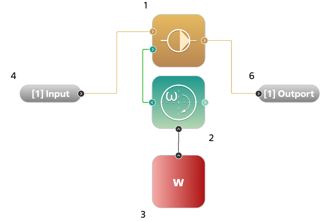
Fig. 2 Variable w

 The flow rate is measured by a mass flow sensor at the very exit of the system (in Fig. 1 - on the right). For this flow rate, the Outport block is set with the variable name m. It will be used in further optimization as the target variable.

2.  Statement of the optimization problem

 Let \(m(w)\) be the mass flow rate at the outlet of the industrial circuit at the angular velocity of the pump \(w\). It is required to find a value of \(w^*\) at which the flow rate is equal to the given value (1) :

(1)\[{m}(w^*) = M_{\text{target}}, \quad M_{\text{target}} = 326.6\ \text{кг/с}\]

 The equation (2) is solved:

(2)\[m(w) - 326.6 = 0\]

 To apply numerical optimizers, we reformulate this into the problem of minimizing the square of the residual (3) :

(3)\[\min_{w} F(w), \quad F(w) = \bigl( {m}(w) - 326.6 \bigr)^2\]

 When the function \(m(w)\) is monotonic (which is typical for a centrifugal pump), \(F(w)\) has a single global minimum (equal to 0) at the point \(w^*\).

 Physical limitations on pump rotation speed (rad/s) (4) :

(4)\[w_{\min} = 140, \quad w_{\max} = 200\]

 They are found empirically, since the function \(m(w)\) is monotone.

3.  Selection of optimization methods

3.1.  Brent’s Method for Finding Roots

The root_scalar method with the brentq parameter implements the classic Brent root-finding method.

The principle of searching for the root

 When using this method, we will look for the root of the equation (5) :

(5)\[m(w) - 326.6 = 0\]

Note

The method requires that the function have opposite signs at the ends of the interval (for our monotonic dependence this is the case).

 The algorithm does not select one method, but dynamically combines three at once depending on the situation:

1. Inverse quadratic interpolation: This is the main “accelerator” of the method. When we have three points with their values, the algorithm constructs a parabola through them, not from x to y, but from y to x. It then finds where y=0 and gets a very good approximation of the root, allowing the method to converge very quickly on smooth functions. Fig. 3 shows the formula for this inverse interpolation:

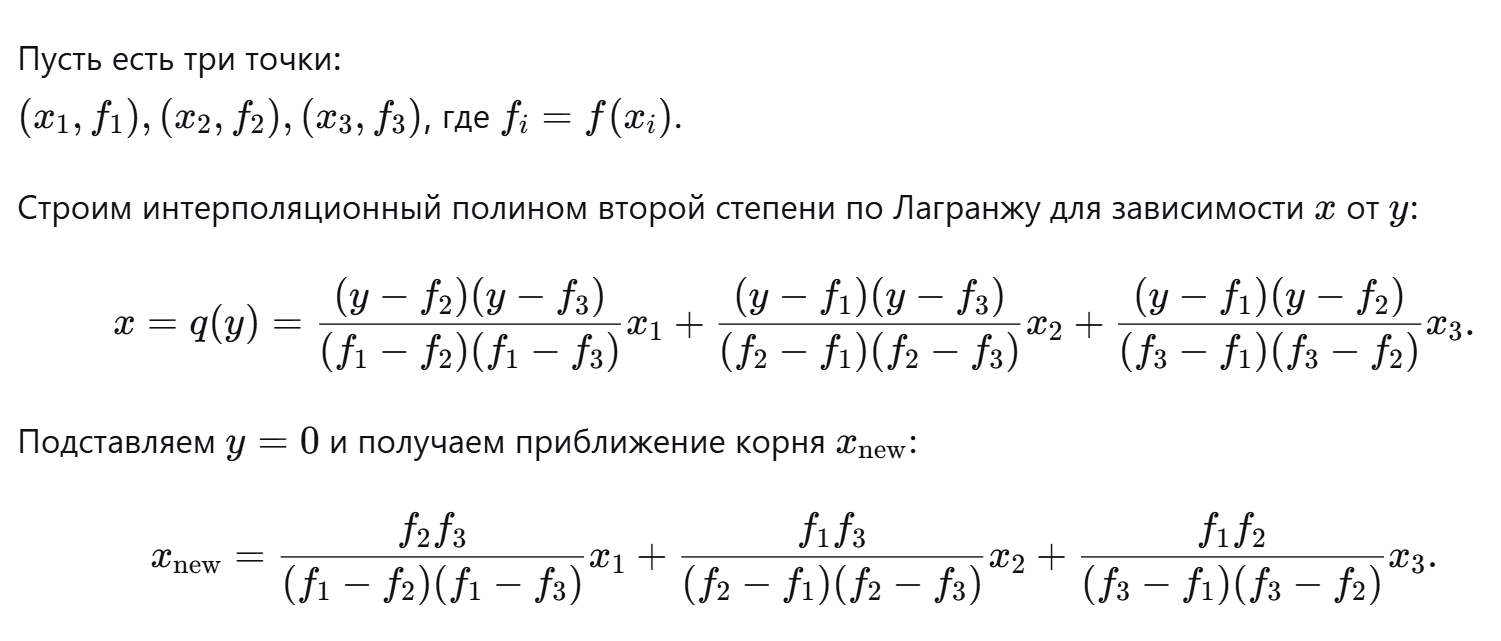
Fig. 3 Formula for inverse interpolation

2. Secant Method: Brent uses this method when he only has two points to interpolate. This is also a fast method, but it is less robust than inverse quadratic interpolation.

3. Method of dividing a segment in half: This is the “safety net” of the algorithm. If quick but risky steps (interpolation or secant) lead to a point that doesn’t guarantee a reliable root capture, the algorithm takes one guaranteed step, simply dividing the current root interval in half. This ensures that the root interval will continue to decrease, and the algorithm will never “lose” the root.

3.2.  Brent’s Optimization Method

 For solving one-dimensional optimization problems on a segment, the combined Brent method is most often recommended. It offers the best balance of reliability and speed for most practical problems.

 Let’s look at why this is so and examine the strengths of each method so you can make an informed choice.

 This method is the de facto standard in most computational libraries (e.g., scipy.optimize.minimize_scalar, MATLAB). It is a hybrid approach that combines the strengths of two methods:

• The golden ratio method guarantees convergence.

• Parabola Method – ensures speed on smooth areas.

How the Golden Ratio Method Works

1. The golden ratio is the division of a segment into two unequal parts so that the ratio of the entire segment to the larger part is equal to the ratio of the larger part to the smaller part (6) :

(6)\[\frac{b-a}{\tau\cdot(b-a)} = \frac{\tau \cdot(b-a)}{(1-\tau)\cdot(b-a)} \quad \Rightarrow \quad \tau = \frac{\sqrt{5}-1}{2} \approx 0.618\]

 The constant \( au\) is called the golden ratio. With this choice, the division points have an important property: one of the interior points calculated in the current step becomes an interior point in the next step, allowing the previously calculated function value to be reused.

2. Step algorithm:

• We set the initial interval [a, b].

• We calculate two interior points:

\(x_1 = a + (1-\tau)(b-a) \quad \text{(left point)}\)

\(x_2 = a + \tau(b-a) \quad \text{(right point)}\)

• We calculate the values ​​of the functions \(f(x_1)\) and \(f(x_2)\).

  • If \(f(x_1) < f(x_2)\), then the minimum is in \([a, x_2]\); the new interval is \([a, x_2]\).

  • If \(f(x_1) \ge f(x_2)\), then the minimum is in \([x_1, b]\); the new interval is \([x_1, b]\).

  • At each step, the interval decreases by \(\tau \approx 1.618\) times.

  • The process is repeated until the required accuracy along the interval length is achieved.

How does the Brent method work

1. First, it tries to approximate the function with a parabola through three points.

2. If the approximation is successful and leads to a rapid descent to the minimum, a parabolic step is used.

3. If the parabola starts to behave unstable at some point, the algorithm automatically switches to the golden section method to ensure that the minimum is not lost and the search continues.

Why is it the best choice

 The combination of the two approaches makes the Brent method simultaneously:

• Very fast (thanks to parabolic interpolation);

• Exceptionally reliable (thanks to the golden ratio).

3.3.  Nelder-Mead Method

The Nelder–Mead method, also known as the deformable polyhedron method and the simplex method, is a method for unconstrained optimization of a function of several variables that does not use the derivative (or more precisely, gradients) of the function and is therefore easily applicable to non-smooth and/or noisy functions.

 The essence of the method lies in the sequential displacement and deformation of the simplex around the extremum point.

Operating principle

 The Nelder-Mead algorithm (the deformable polyhedron method) consists of constructing a simplex and then deforming it in the direction of the minimum using four operations (see Fig. 4 below):

1. Reflection

2. Expansion

3. Contraction - can be external and internal

4. Shrinkage - also called contraction

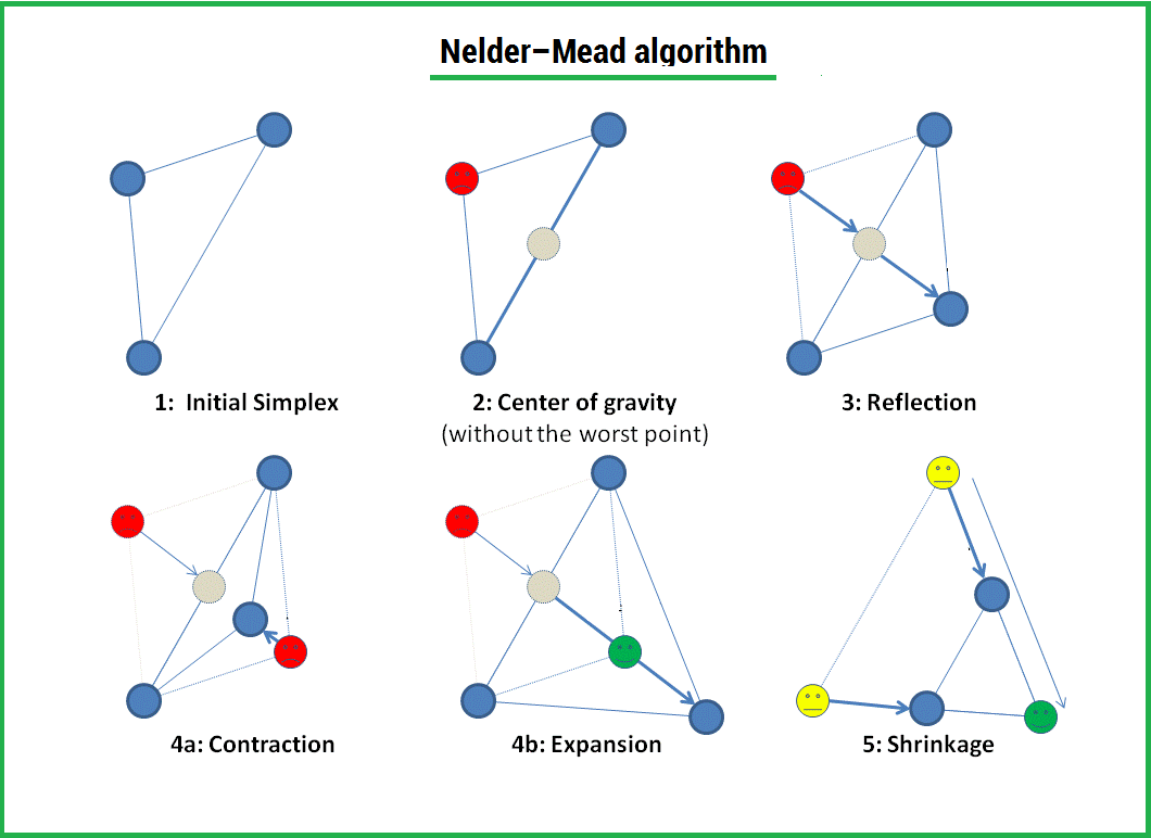
Fig. 4 Nelder-Mead algorithm

 A simplex is a geometric figure that is an n-dimensional generalization of a triangle. For one-dimensional space, it is a segment, for two-dimensional space, it is a triangle. Thus, an n-dimensional simplex has n+1 vertices.

 Algorithm (one iteration):

1. The centroid (arithmetic mean) of all vertices is calculated, except the worst (the one where the function value is maximum).

2. The worst point is successively subjected to deformation operations in the following order:

   • Reflection is a mirror image of the worst vertex relative to the centroid.

   • Depending on the value of the function at the reflected point, the algorithm decides:

     • if the reflected point is better than the best → stretch;

     • if the reflected point is average (between the best and the worst) → external compression;

     • if the reflected point is worse than the worst → internal compression;

     • if compression did not produce improvement → reduction (compression of the entire simplex to the best vertex).

 The diagram(#title5) shows all four basic operations: the centroid is indicated by a gray dot, the worst vertex is indicated by a red one.

Note

The operation that produces the smallest value of the function within a certain logic is performed (not a simple enumeration, but branching).

 Stopping conditions (any of them):

1. The specified maximum number of iterations has been completed.

2. The characteristic size of a simplex (for example, the maximum distance between vertices or the volume) has become smaller than the specified value xatol.

3. The function value at the best vertex changed by less than fatol over several iterations (the required accuracy of the function was achieved).

Note

The Nelder-Mead method is a direct optimization method (zero-order)—it does not require derivative calculations. Convergence is not guaranteed for all functions, but in practice it is often effective, especially for low-dimensional problems (usually \(n \le 20\)).

3.4.  L-BFGS-B Method

L-BFGS-B is an improved version of the classical gradient descent.

Limitations of the method

• Function requirement: The objective function must be smooth and differentiable. L-BFGS-B computes and actively uses the gradient. For nonsmooth or noisy functions, there are more robust direct methods, such as the previously mentioned Nelder-Mead method.

• Finding a local minimum: Like most gradient-based methods, L-BFGS-B finds a local minimum.

Note

L-BFGS-B is the gold standard for problems where the function is smooth, the number of parameters ranges from hundreds to millions, but there are simple constraints on their values.

3.5.  Which method to choose

 If we consider the given optimization problem, then the fastest of the methods that do not require a derivative is Brent’s algorithm for finding a root, since in the problem we have one parameter and a simple monotonic dependence of the flow rate on the frequency (this dependence is very often encountered in various physical models, for example: heat flow on the emissivity or thermal resistance, etc.) and there is a given target flow rate value, so we can directly search for the root of the equation, rather than minimizing a quadratic function as in the other three methods. This method allows you to quickly select the optimal parameter value for such simple tasks.

 Brent’s optimization method is also applicable to this problem, but it turns out to be slower than the classical root finding method. It is recommended for use when it is not possible to easily find the root of the original equation (the function has the same signs at the ends of the interval, the function is not monotonic, the equation cannot be written because the target value is not given, and the task is minimization, etc.).

 For more complex optimization problems, where there are several parameters (2–10) and an unknown dependence, it is recommended to use the Nelder-Mead method.

 If the objective function is smooth and differentiable with respect to all parameters, which is often the case in physical models, and it is possible to set the boundaries of the change in variables, then the L-BFGS-B algorithm can be used, which will be faster than the Nelder-Mead method.

3.6.  Comparison of methods for a given task

• Comparison 1, Fig. 5:

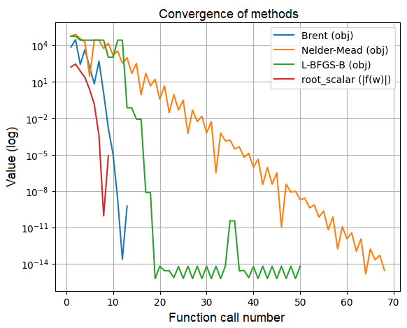
Fig. 5 Comparison 1

• Comparison 2, Fig. 6:

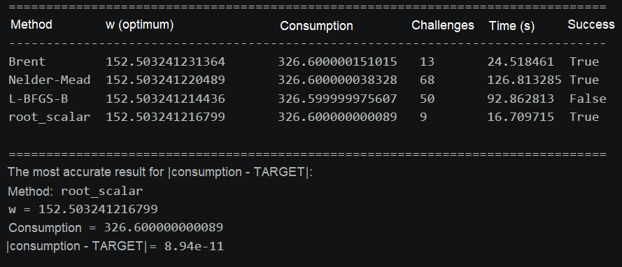
Fig. 6 Comparison 2

 As can be seen, all methods yielded the same optimal frequency value with an accuracy of up to 7 decimal places. Brent’s root-finding method showed the fastest convergence rate.

4.  Code for applying methods

 First, the common code section for all methods is presented. This includes connecting to the model on the REPEAT VISION platform, initializing the target value and necessary functions, etc. Before running, you need to insert your api token and project ID, and specify your simulation time in [ms] in t_interval.

import repeat as rp
import pandas as pd
import numpy as np
import matplotlib.pyplot as plt
from scipy.optimize import minimize, minimize_scalar, root_scalar
import time

user = rp.User(token = "TOKEN") #API
app = rp.Application(user)
project = 'ID'
t_interval = rp.TimeInterval(start = 0, end = 15000)
model = app.get_exploration_model(project, t_interval)

TARGET = 326.6   # целевой расход
bounds = [(140.0, 200.0)]   # границы
w0 = 130.0   # ваше начальное приближение
HIGH_PRECISION = {  # параметры оптимизаторов
    'Nelder-Mead':   {'maxiter': 1000, 'xatol': 1e-8, 'fatol': 1e-8, 'disp': False},
    'L-BFGS-B':      {'maxiter': 1000, 'gtol': 1e-8, 'disp': False},
    'Brent':         {'maxiter': 1000, 'xatol': 1e-8, 'fatol': 1e-8},
    'root_scalar':   {'maxiter': 1000, 'xtol': 1e-8, 'rtol': 1e-8}
}


def result(w, model):
    v1 = model.existing_variables.copy()
    v2 = v1.copy()
    v2['w'] = w

    with model as md:
        md.run(v2)
        m = md.get_results('m')

    results = {
        'm': m
    }

    return results


def get_rashod(w):
    def run_simulation():
        with model as md:
            model_data = result(w, md)
            rashod_val = model_data["m"].to_numpy()[-1]
            return rashod_val


    return run_simulation()


def objective(w):
    r = get_rashod(w)
    obj = (r - TARGET) ** 2
    return obj


def root_function(w):
    r = get_rashod(w)
    f_val = r - TARGET
    return f_val

• Line 14. Target expense.

• Line 15. Boundaries.

• Line 16 Your initial guess.

• Line 17. Optimizer parameters.

• Lines 26-28. We obtain a vector of flow values ​​over time (for optimization, we take the last value of this vector).

• Lines 42-46. Runs the model with parameter w and returns the flow rate at the end of the interval.

• Lines 52-55. Returns the objective function (squared error).

• Lines 58-61. Returns the equation for finding the root.

 Now let’s move on to the code snippets for each of the methods (it should be inserted after the general code snippet):

4.1.  Brent’s method for finding the root

opt_result = root_scalar(
            root_function,
            method='brentq',
            bracket=(bounds[0][0], bounds[0][1]),
            options={'maxiter': HIGH_PRECISION['root_scalar']['maxiter'],
                     'xtol': HIGH_PRECISION['root_scalar']['xtol'],
                     'rtol': HIGH_PRECISION['root_scalar']['rtol']}
        )

optimal_w = opt_result.root
optimal_rashod = get_rashod(optimal_w)
print(f"\nОптимум: w = {optimal_w:.4f}, расход = {optimal_rashod:.4f} (цель {TARGET})")

4.2.  Brent’s optimization method

opt_result = minimize_scalar(
    objective,
    w0,
    method='bounded',
    bounds=(bounds[0][0], bounds[0][1]),
    options=HIGH_PRECISION['Brent']
)
optimal_w = opt_result.x
optimal_rashod = get_rashod(optimal_w)
print(f"\nОптимум: w = {optimal_w:.4f}, расход = {optimal_rashod:.4f} (цель {TARGET})")

4.3.  Nelder-Mead method

opt_result = minimize(
    objective,
    w0,
    method='Nelder-Mead',
    bounds=bounds,
    options=HIGH_PRECISION['Nelder-Mead']
)
optimal_w = opt_result.x[0]
optimal_rashod = get_rashod(optimal_w)
print(f"\nОптимум: w = {optimal_w:.4f}, расход = {optimal_rashod:.4f} (цель {TARGET})")

4.4.  L-BFGS-B Method

opt_result = minimize(
    objective,
    w0,
    method='L-BFGS-B',
    bounds=bounds,
    options=HIGH_PRECISION['L-BFGS-B']
)
optimal_w = opt_result.x[0]
optimal_rashod = get_rashod(optimal_w)
print(f"\nОптимум: w = {optimal_w:.4f}, расход = {optimal_rashod:.4f} (цель {TARGET})")

4.5.  The advantages of implementing optimization in Python over built-in algorithms on the REPEAT VISION platform

1. Flexibility in choosing and customizing methods:

   • The REPEAT VISION platform offers a fixed set of algorithms with a limited number of parameters.

   • Python + SciPy/NumPy give access to dozens of methods and full control over their hyperparameters (precision, maximum number of iterations, tolerances, etc.).

2. Visualization of the optimization process:

   • The REPEAT VISION platform displays only the final result. Python allows you to plot convergence graphs (function value versus iteration number), trajectories in parameter space, simplex evolution, and call histograms.

   • This helps us understand why the algorithm stopped, whether it got stuck in a local minimum, or whether the step size decreased too quickly. Visualization is a powerful tool for diagnostics and fine-tuning.

3. Collection and analysis of diagnostic information:

   • In Python, it is easy to store a complete history of function calls, gradient values, and the time of each step.